
4.3: Interpreting the Graph of a Function


- Last updated
- Jan 4, 2021
- Save as PDF
( \newcommand{\kernel}{\mathrm{null}\,}\)
In the previous section, we began with a function and then drew the graph of the given function. In this section, we will start with the graph of a function, then make a number of interpretations based on the given graph: function evaluations, the domain and range of the function, and solving equations and inequalities.
The Vertical Line Test
Consider the graph of the relation R shown in Figure 4.3.1(a). Recall that we earlier defined a relation as a set of ordered pairs. Surely, the graph shown in Figure 4.3.1(a) is a set of ordered pairs. Indeed, it is an infinite set of ordered pairs, so many that the graph is a solid curve.
In Figure 4.3.1(b), note that we can draw a vertical line that cuts the graph more than once. In Figure 4.3.1(b), we’ve drawn a vertical line that cuts the graph in two places, once at (x,y1), then again at (x,y2), as shown in Figure 4.3.1(c). This means that the domain object x is paired with two different range objects, namely y1 and y2, so relation R is not a function.
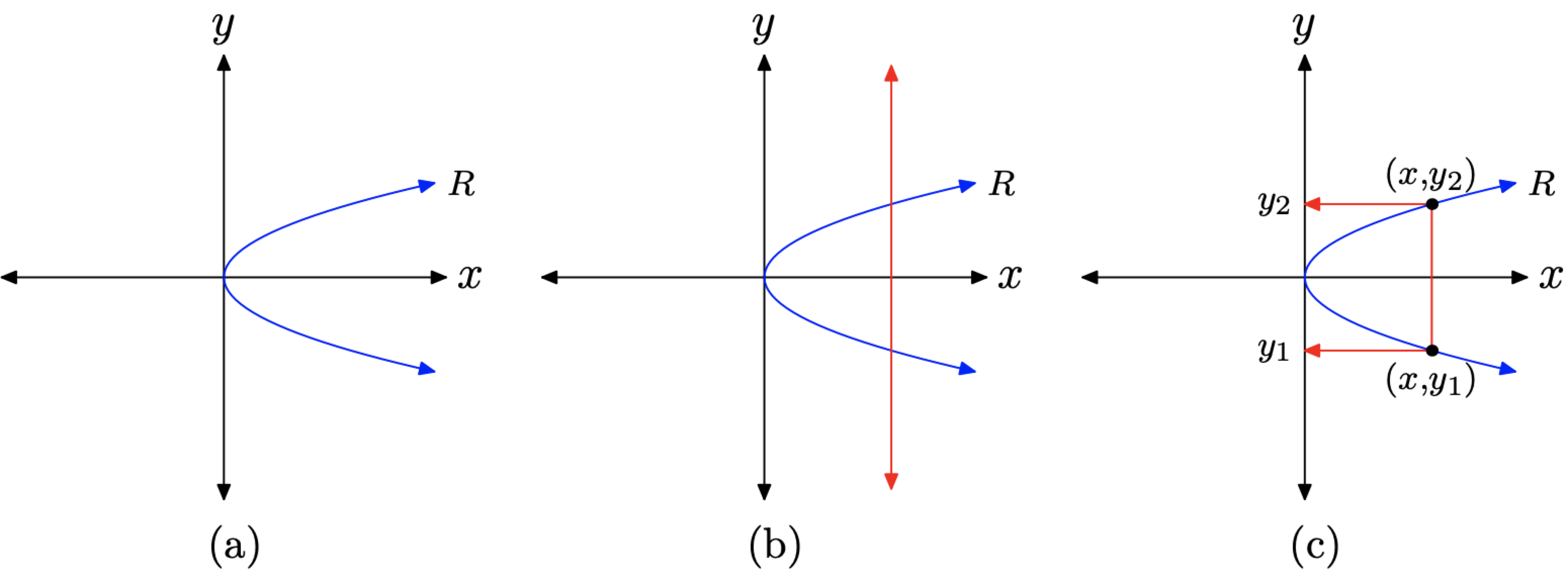
Figure 4.3.1. Explaining the vertical line test for functions.
Recall the definition of a function.
A relation is a function if and only if each object in its domain is paired with one and only one object in its range.
Consider the mapping diagram in Figure 4.3.2, where we’ve used arrows to indicate the ordered pairs (x,y1) and (x,y2) in Figure 4.3.1(c). Note that x, an object in the domain of R, is mapped to two objects in the range of R, namely y1 and y2. Hence, the relation R is not a function.
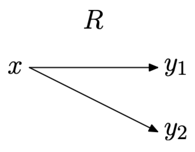
Figure 4.3.2. A mapping diagram representing the points (x,y1) and (x,y2) in Figure 4.3.1(c).
This discussion leads to the following result, called the vertical line test for functions.
If any vertical line cuts the graph of a relation more than once, then the relation is NOT a function.
Hence, the circle pictured in Figure 4.3.3(a) is a relation, but it is not the graph of a function. It is possible to cut the graph of the circle more than once with a vertical line, as shown in Figure 4.3.3(a). On the other hand, the parabola shown in Figure 4.3.3(b) is the graph of a function, because no vertical line will cut the graph more than once.
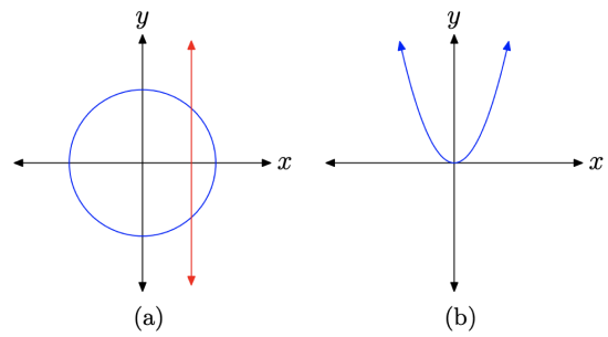
Figure 4.3.3. Use the vertical line test to determine if the graph is the graph of a function.
Reading the Graph for Function Values
We know that the graph of f pictured in Figure 4.3.4 is the graph of a function. We know this because no vertical line will cut the graph of f more than once.
We earlier defined the graph of f as the set of all ordered pairs (x,f(x)), so that x is in the domain of f. Consequently, if we select a point P on the graph of f, as in Figure 4.3.4(a), we label the point P(x, f(x)). However, we can also label this point as P(x,y), as shown in Figure 4.3.4(b). This leads to a new interpretation of f(x) as the y-value of the point P. That is, f(x) is the y-value that is paired with x.
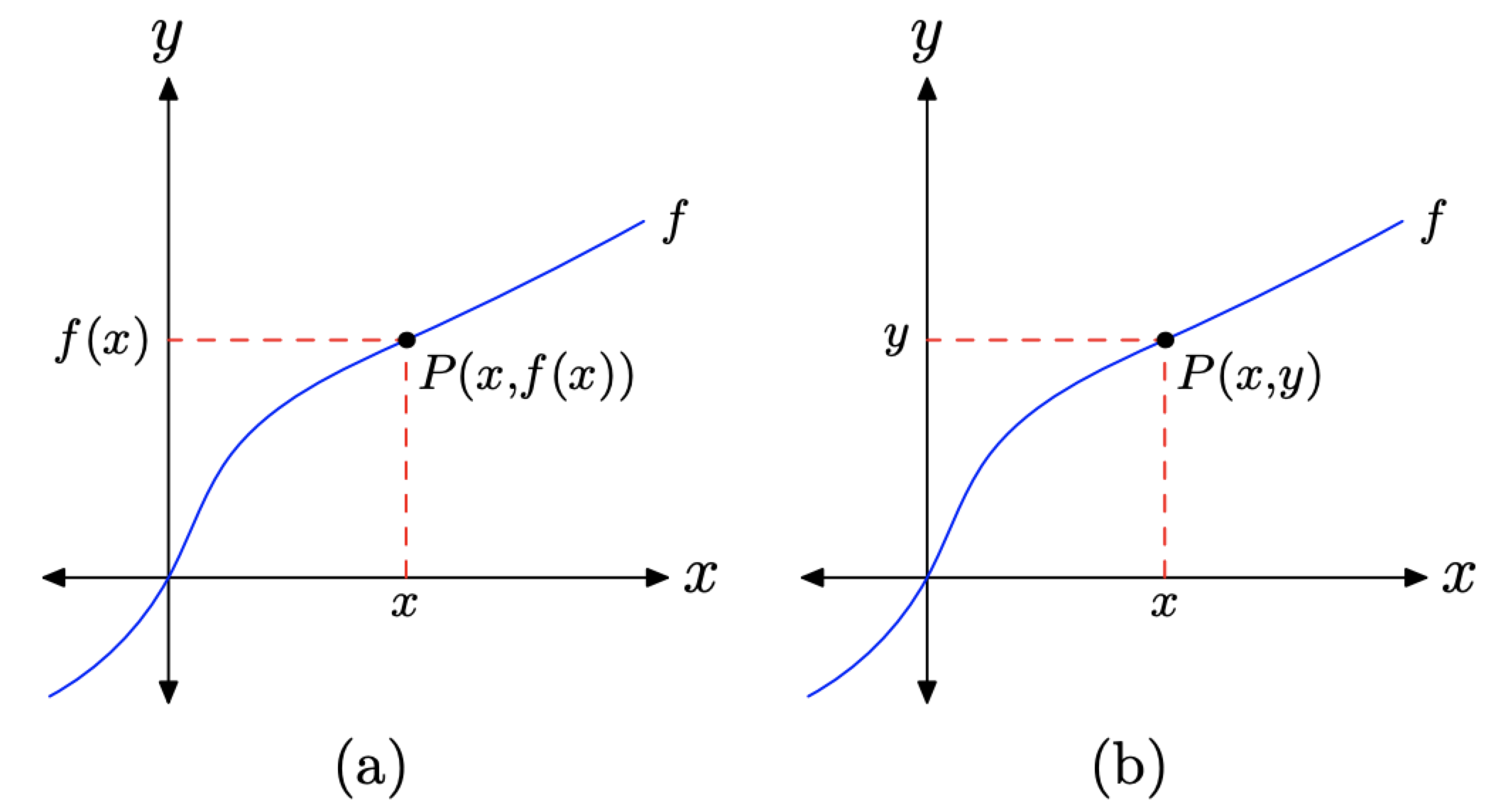
Figure 4.3.4. Reading the graph of a function.
f(x) is the y-value that is paired with x.
Two more comments are in order. In Figure 4.3.4(a), we select a point P on the graph of f.
- To find the x-value of the point P, we must project the point P onto the x-axis.
- To find f(x), the value of y that is paired with x, we must project the point P onto the y-axis.
Let’s look at an example.
Given the graph of f in Figure 4.3.5(a), find f(4).
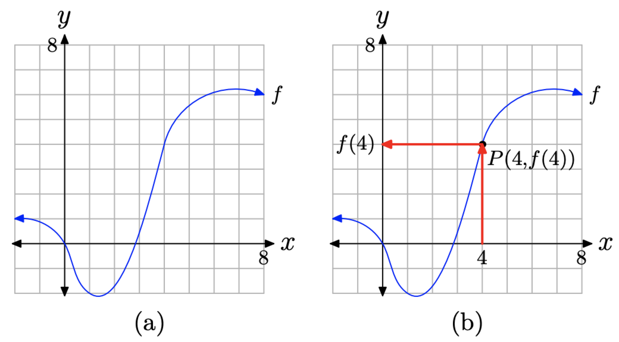
Figure 4.3.5. Finding the value of f(4).
Solution
First, note that the graph of f represents a function. No vertical line will cut the graph of f more than once.
Because f(4) represents the y-value that is paired with an x-value of 4, we first locate 4 on the x-axis, as shown in Figure (\PageIndex{5}\)(b). We then draw a vertical arrow until we intercept the graph of f at the point P(4, f(4)). Finally, we draw a horizontal arrow from the point P until we intercept the y-axis. The projection of the point P onto the y-axis is the value of f(4).
Because we have a grid that shows a scale on each axis, we can approximate the value of f(4). It would appear that the y-value of point P is approximately 4. Thus, f(4)≈4.
Let’s look at another example.
Given the graph of f in Figure 4.3.6(a), find f(5).
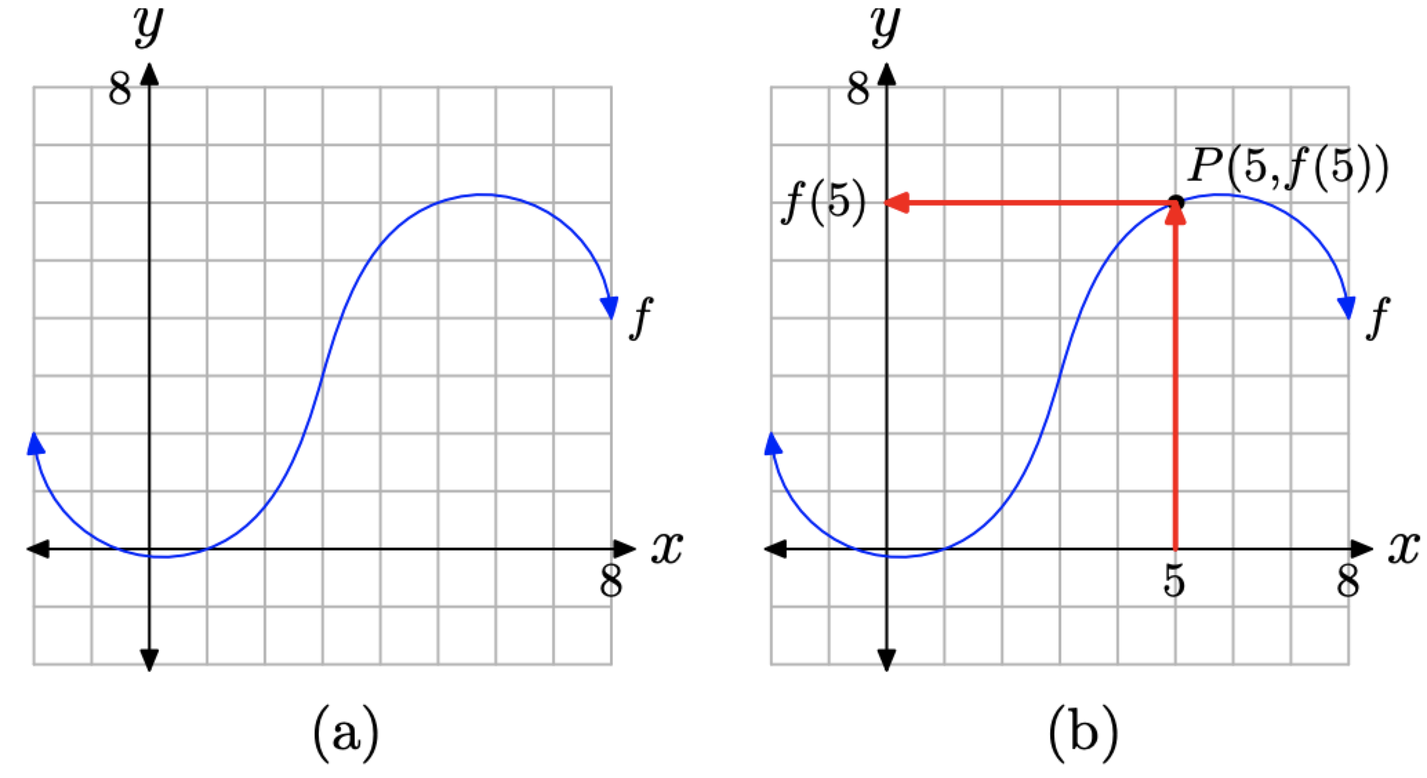
Figure 4.3.6. Finding the value of f(5).
Solution
First, note that the graph of f represents a function. No vertical line will cut the graph of f more than once.
Because f(5) represents the y-value that is paired with an x-value of 5, we first locate 5 on the x-axis, as shown in Figure 4.3.6(b). We then draw a vertical arrow until we intercept the graph of f at the point P(5, f(5)). Finally, we draw a horizontal arrow from the point P until we intercept the y-axis. The projection of the point P onto the y-axis is the value of f(5).
Because we have a grid that shows a scale on each axis, we can approximate the value of f(5). It would appear that the y-value of point P is approximately 6. Thus, f(5)≈6.
Let’s reverse the interpretation in another example.
Given the graph of f in Figure 4.3.7(a), for what value of x does f(x) = −4?
Solution
Again, the graph in Figure 4.3.7 passes the vertical line test and represents the graph of a function.
This time, in the equation f(x)=−4, we’re given a y-value equal to −4. Consequently, we must reverse the process used in Example 4.3.1 and Example 4.3.2. We first locate the y-value −4 on the y-axis, then draw a horizontal arrow until we intercept
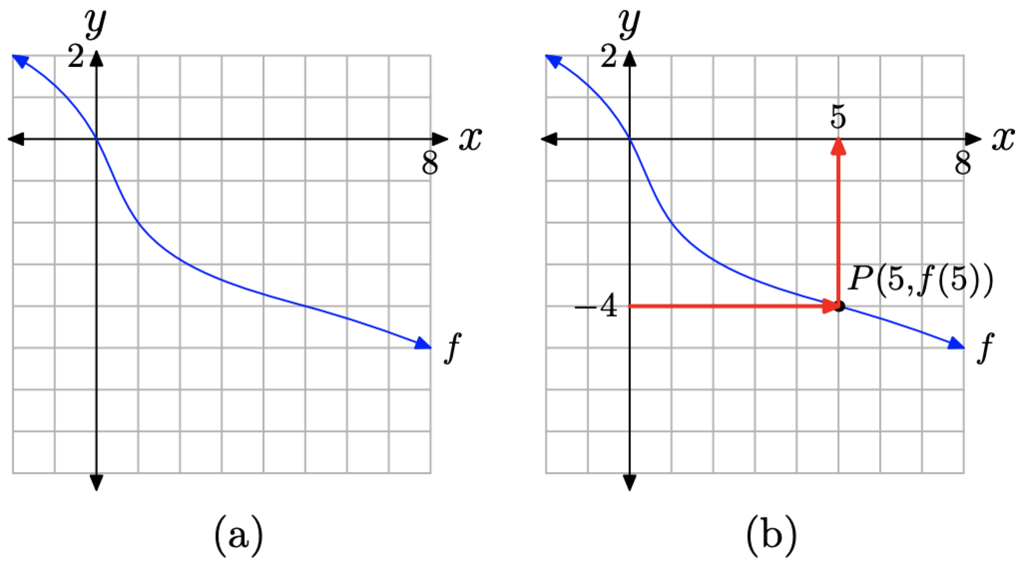
Figure 4.3.7. Finding x so that f(x)=−4.
the graph of f at P, as shown in Figure 4.3.7(b). Finally, we draw a vertical arrow from the point P until we intercept the x-axis. The projection of the point P onto the x-axis is the solution of f(x)=−4.
Because we have a grid that shows a scale on each axis, we can approximate the x-value of the point P. It seems that x≈5. Thus, we label the point P(5, f(5)), and the solution of f(x)=−4 is approximately x≈5.
This solution can easily be checked by computing f(5). Simply start with 5 on the x-axis, then reverse the order of the arrows shown in Figure 4.3.7(b). You should wind up at −4 on the y-axis, demonstrating that f(5)=−4.
The Domain and Range of a Function
We can use the graph of a function to determine its domain and range. For example, consider the graph of the function shown in Figure 4.3.8(a).
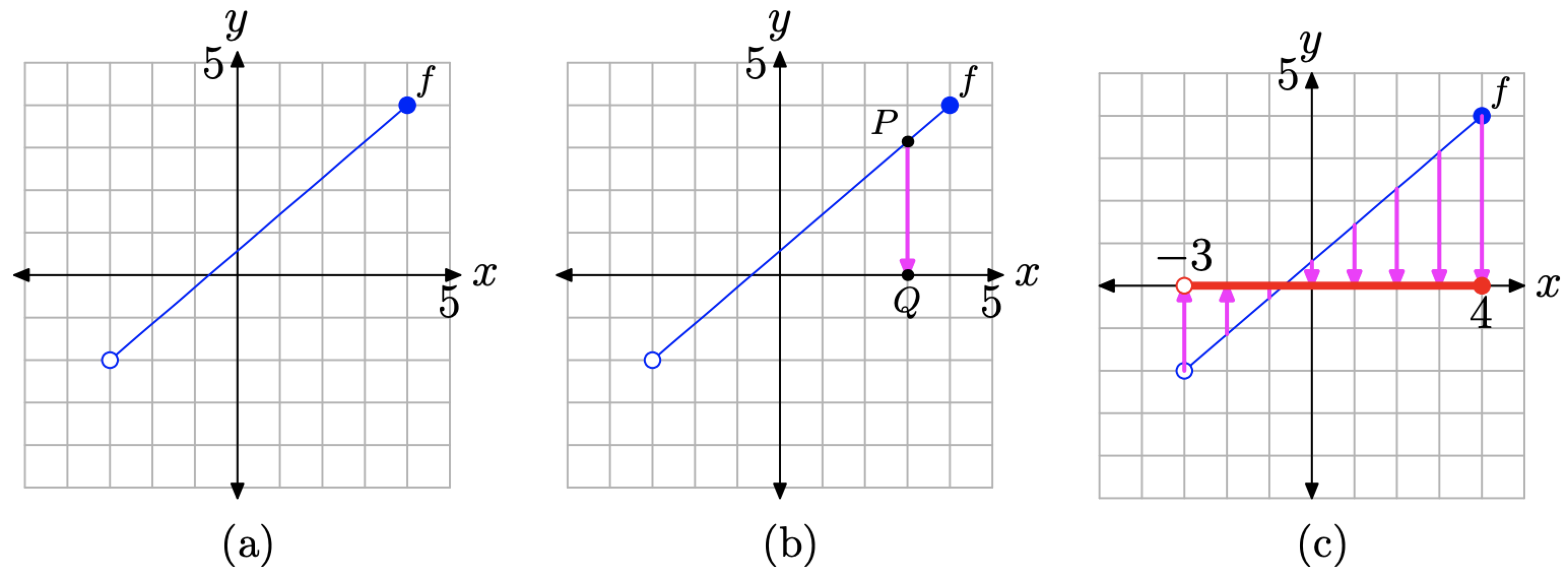
Figure 4.3.8. Determining the domain of a function from its graph.
Note that no vertical line will cut the graph of f more than once, so the graph of f represents a function.
To determine the domain, we must collect the x-values (first coordinates) of every point on the graph of f. In Figure 4.3.8(b), we’ve selected a point P on the graph of f, which we then project onto the x-axis. The image of this projection is the point Q, and the x-value of the point Q is an element in the domain of f.
Think of the projection shown in Figure 4.3.8(b) in the following manner. Imagine a light source above the point P. The point P blocks out the light and its shadow falls onto the x-axis at the point Q. That is, think of point Q as the “shadow” that the point P produces when it is projected vertically onto the x-axis.
Now, to find the domain of the function f, we must project each point on the graph of f onto the x-axis. Here’s the question: if we project each point on the graph of f onto the x-axis, what part of the x-axis will “lie in shadow” when the process is complete? The answer is shown in Figure 4.3.8(c).
In Figure 4.3.8(c), note that the “shadow” created by projecting each point on the graph of f onto the x-axis is shaded in red (a thicker line if you are viewing this in black and white). This collection of x-values is the domain of the function f. There are three critical points that we need to make about the “shadow” on the x-axis in Figure 4.3.8(c).
- All points lying between x=−3 and x=4 have been shaded on the x-axis in red.
- The left endpoint of the graph of f is an open circle. This indicates that there is no point plotted at this endpoint. Consequently, there is no point to project onto the x-axis, and this explains the open circle at the left end of our “shadow” on the x-axis.
- On the other hand, the right endpoint of the graph of f is a filled endpoint. This indicates that this is a plotted point and part of the graph of f. Consequently, when this point is projected onto the x-axis, a shadow falls at x = 4. This explains the filled endpoint at the right end of our “shadow” on the x-axis.
We can describe the x-values of the “shadow” on the x-axis using set-builder notation.
Domain of f={x:−3<x≤4}
Note that we don’t include −3 in this description because the left end of the shadow on the x-axis is an empty circle. Note that we do include 4 in this description because the right end of the shadow on the x-axis is a filled circle.
We can also describe the x-values of the “shadow” on the x-axis using interval notation.
Domain of f=(−3,4]
We remind our readers that the parenthesis on the left means that we are not including −3, while the bracket on the right means that we are including 4.
To find the range of the function, picture again the graph of f shown in Figure 4.3.9(a). Proceed in a similar manner, only this time project points on the graph of f onto the y-axis, as shown in Figures 4.3.9(b) and (c).
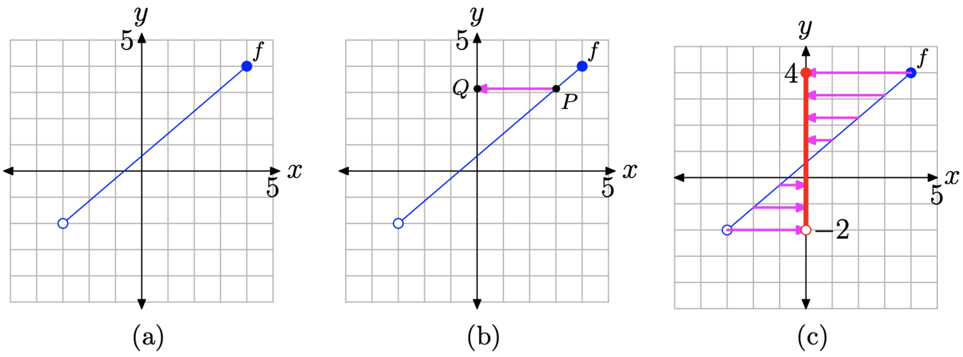
Figure 4.3.9. Determining the range of a function from its graph.
Note which part of the y-axis “lies in shadow” once we’ve projected all points on the graph of f onto the y-axis.
- All points lying between y=−2 and y=4 have been shaded on the y-axis in red (a thicker line style if you are viewing this in black and white).
- The left endpoint of the graph of f is an empty circle, so there is no point to project onto the y-axis. Consequently, there is no “shadow” at y=−2 on the y-axis and the point is left unshaded (an empty circle).
- The right endpoint of the graph of f is a filled circle, so there is a “shadow” at y=4 on the y-axis and this point is shaded (a filled circle).
We can now easily describe the range in both set-builder and interval notation.
Range of f=(−2,4]={y:−2<y≤4}
Let’s look at another example.
Use set-builder and interval notation to describe the domain and range of the function represented by the graph in Figure 4.3.10(a).
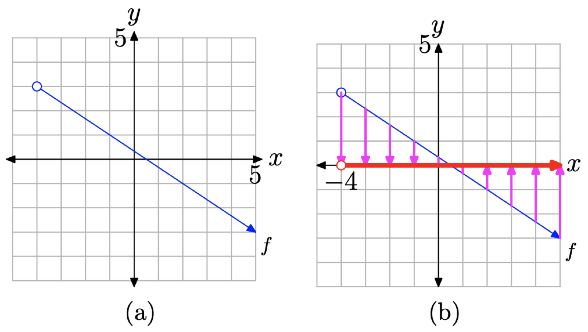
Figure 4.3.10. Determining the domain from the graph of f.
Solution
To determine the domain of f, project each point on the graph of f onto the x-axis. This projection is indicated by the “shadow” on the x-axis in Figure 4.3.10(b). Two important points need to be made about this “shadow” or projection.
1. The left endpoint of the graph of f is empty (indicated by the open circle), so it has no projection onto the x-axis. This is indicated by an open circle at the left end (at x=−4) of the “shadow” or projection on the x-axis.
2. The arrowhead on the right end of the graph of f indicates that the graph of f continues downward and to the right indefinitely. Consequently, the projection onto the x-axis is a shadow that moves indefinitely to the right. This is indicated by an arrowhead at the right end of the “shadow” or projection on the x-axis.
Consequently, the domain of f is the collection of x-values represented by the “shadow” or projection onto the x-axis. Note that all x-values to the right of x=−4 are shaded on the x-axis. Consequently,
Domain of f=(−4,∞)={x:x>−4}
To find the range, we must project each point on the graph of f (redrawn in Figure 4.3.11(a)) onto the y-axis. The projection is indicated by a “shadow” or projection on the y-axis, as seen in Figure 4.3.11(b). Two important points need to be made about this “shadow” or projection.
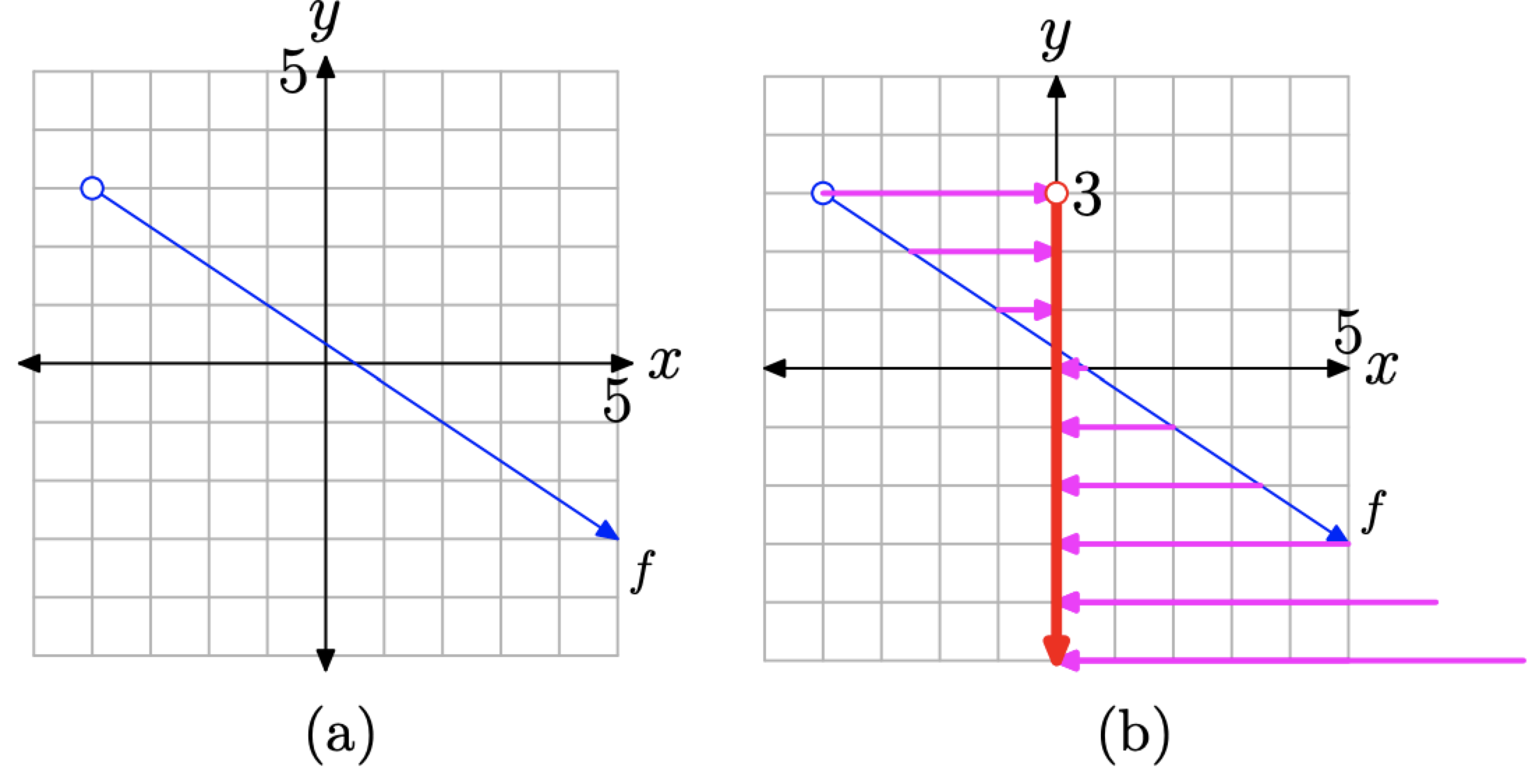
Figure 4.3.11. Determining the range from the graph of f.
- The left endpoint of the graph of f is empty (indicated by an open circle), so it has no projection onto the y-axis. This is indicated by an open circle at the top end (at y=3) of the “shadow” on the y-axis.
- The arrowhead on the right end of the graph of f indicates that the graph of f continues downward and to the right indefinitely. Consequently, the projection of the graph of f onto the y-axis is a shadow that moves indefinitely downward. In Figure 4.3.11(b), note how projections of points on the graph of f not visible in the viewing window come in from the lower right corner and cast “shadows” on the y-axis.
Consequently, the range of f is the collection of y-values shaded on the y-axis of the coordinate system shown in Figure 4.3.11(b). Note that all y-values lower than y=3 are shaded on the y-axis. Thus, the range of f is
Range of f=(−∞,3)={y:y<3}
Let’s look at another example.
Use set-builder and interval notation to describe the domain and range of the function represented by the graph in Figure 4.3.12(a).
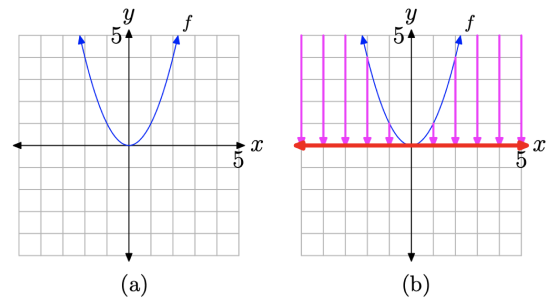
Figure 4.3.12. Determining the domain from the graph of f.
Solution
To determine the domain of f, we must project all points on the graph of f onto the x-axis. This projection is indicated by the red “shadow” (or thicker line style if you are viewing this in black and white) shown on the x-axis in Figure 4.3.12(b). Two important points need to be made about this “shadow” or projection.
- The arrow at the end of the left half of the graph of f in Figure 4.3.12(a) indicates that this half of the graph of f opens indefinitely to the left and upward. Consequently, when the points on the left half of the graph of f are projected onto the x-axis, the “shadow” or projection extends indefinitely to the left. Note how points on the graph that fall outside the viewing window come in from the upper left corner and cast “shadows” on the x-axis.
- The arrow at the end of the right half of the graph of f in Figure 4.3.12(a) indicates that this half of the graph of f opens indefinitely to the right and upward. Consequently, when the points on this half of the graph of f are projected onto the x-axis, the “shadow” or projection extends indefinitely to the right.
Consequently, the entire x-axis lies in “shadow,” making the domain of f to be
Domain of f=(−∞,∞)={x:x∈R}
To determine the range of f, we must project all points on the graph of f onto the y-axis. This projection is indicated by the red “shadow” (or thicker line if you are viewing this in black and white) shown on the y-axis in Figure 4.3.13(b). Two important points need to made about this “shadow” or projection.
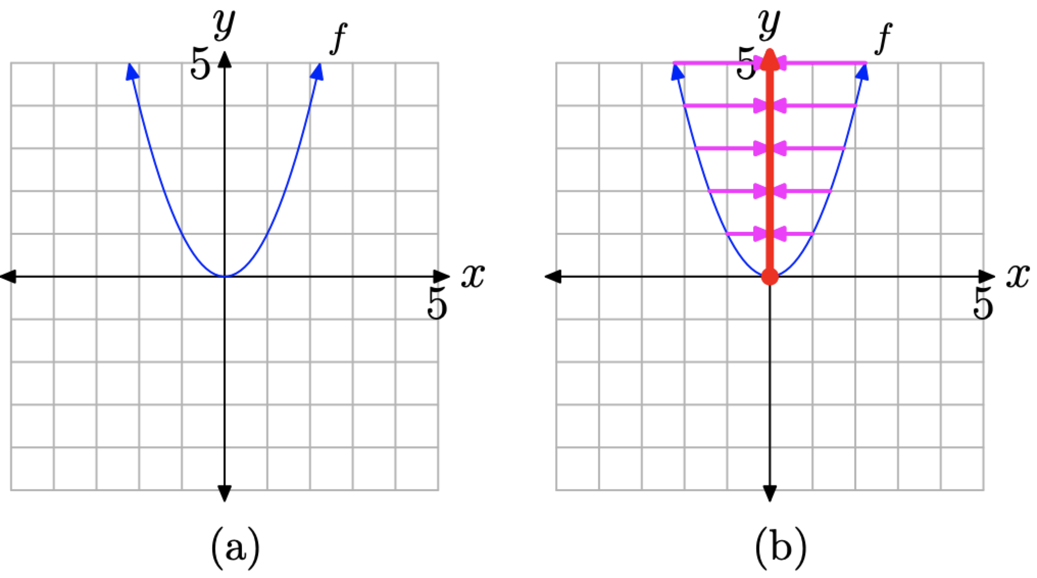
Figure 4.3.13. Determining the range from the graph of f.
- The graph of f passes through the origin (the point (0, 0)). This is the lowest point on the graph and hence its shadow is the endpoint on the low end of the shaded region on the y-axis.
- The arrows at the end of each half of the graph of f indicate that the graph opens upward indefinitely. Hence, when points on the graph of f are projected onto the y-axis, the “shadow” or projection extends upward indefinitely. This is indicated by an arrow on the upper end of the “shadow” on the y-axis.
Consequently, all points on the y-axis above and including the point at the origin “lie in shadow.” Thus, the range of f is
Range of f=[0,∞)={y:y≥0}
Using a Graphing Calculator to Determine Domain and Range
We’ve learned how to find the domain and range of a function by looking at its graph. Therefore, if we define a function by means of an expression, such as f(x)=√4−x, then we should be able to capture the domain and range of f from its graph, provided, of course, that we can draw the graph of f. We’ll find the graphing calculator will be a handy tool for this exercise.
Use set-builder and interval notation to describe the domain and range of the function defined by the rule
f(x)=√4−x
Solution
Load the expression defining f into the Y= menu, as shown in Figure 4.3.14(a). Select 6:ZStandard from the ZOOM menu to produce the graph of f shown in Figure 4.3.14(b).
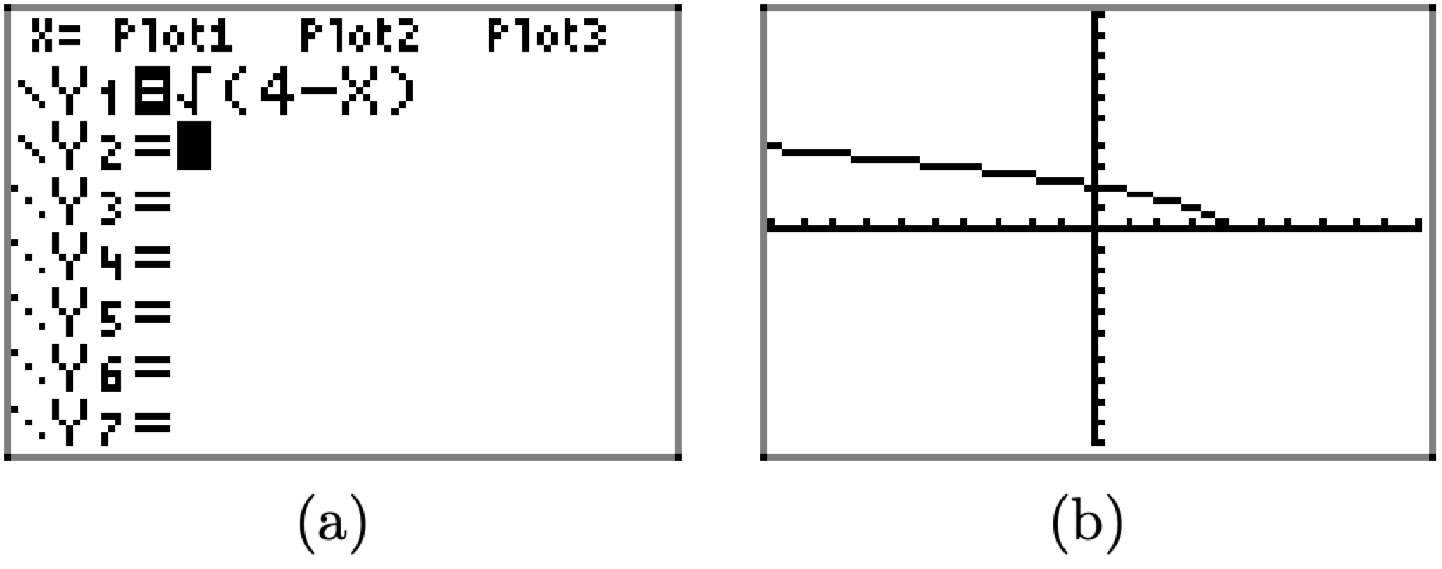
Figure 4.3.14. Sketching the graph of f(x)=√4−x.
Copy the image in Figure 4.3.14(b) onto a sheet of graph paper. Label and scale each axis with the WINDOW parameters xmin, xmax, ymin, and ymax, as shown in Figure 4.3.15(a).
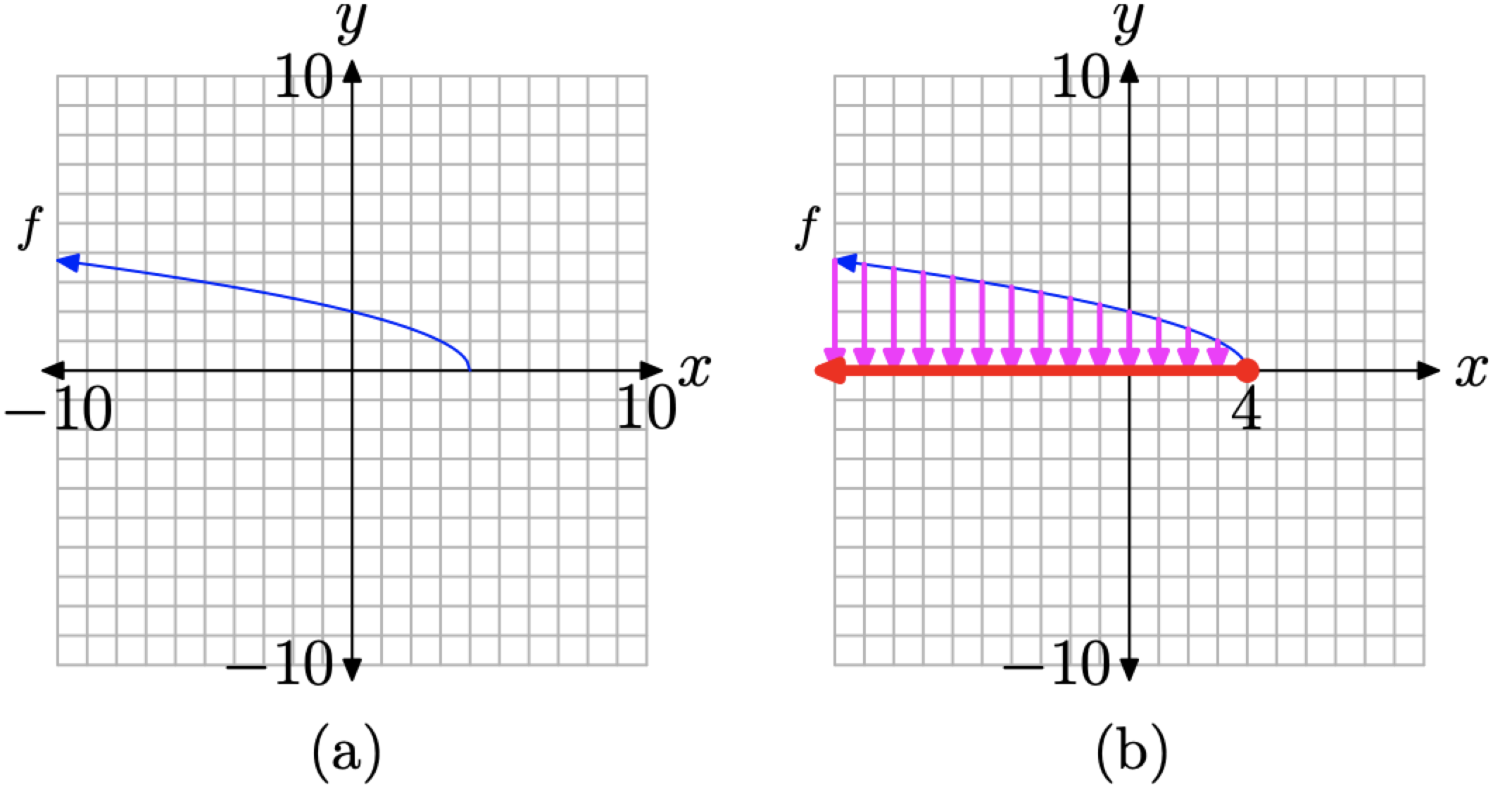
Figure 4.3.15. Capturing the domain of f(x)=√4−x from its graph.
Next, project each point on the graph of f onto the x-axis, as shown in Figure 4.3.15(b). Note that we’ve made two assumptions about the graph of f.
- At the left end of the graph in Figures 4.3.14(b) and 4.3.15(b), we assume that the graph of f continues upward and to the left indefinitely. Hence, the “shadow” or projection onto the x-axis will move indefinitely to the left. This is indicated by attaching an arrowhead to the left-hand end of the region that “lies in shadow” on the x-axis, as shown in Figure 4.3.15(b).
- We also assume that the right end of the graph ends at the point (4,0). This accounts for the “filled dot” when this point on the graph of f is projected onto the x-axis.
Note that the “shadow” or projection onto the x axis in Figure 4.3.15(b) includes all values of x less than or equal to 4. Thus, the domain of f is Domain of f=(−∞,4]={x:x≤4}
We can intuit this result by considering the expression that defines f. That is, consider the rule or definition
f(x)=√4−x
Recall that we earlier defined the domain of f as the set of “permissible” x-values. In this case, it is impossible to take the square root of a negative number, so we must be careful selecting the x-values we use in this rule. Note that x=4 is allowable, as
f(0)=√4−4=√0=0
However, numbers larger than 4 cannot be used in this rule. For example, consider what happens when we attempt to use x=5.
f(x)=√4−5=√−1
We’ll leave it to our readers to test other values of x that are less than 4. They will also produce real answers when they are input into the rule f(x)=√4−x. Note that this also verifies our earlier conjecture that the “shadow” or projection shown in Figure 4.3.15(b) continues indefinitely to the left.
Instead of “guessing and checking,” we can speed up the analysis of the domain of f(x)=√4−x by noting that the expression under the radical must not be a negative number. Hence, 4−x must either be greater than or equal to zero. This argument produces an inequality that is easily solved for x.
4−x≥0−x≥−4x≤4
This last result verifies that the domain of f is all values of x that are less than or equal to 4, which is in complete agreement with the “shadow” or projection onto the x-axis shown in Figure 4.3.15(b).
To determine the range of f, we must project each point on the graph of f onto the y-axis, as shown in Figure 4.3.16(b).
Again, we make two assumptions about the graph of f.
1. At the left-end of the graph of f(x)=√4−x in Figures 4.3.14(b) and 4.3.16(b), we assume that the graph of f continues upward and to the left indefinitely. Thus, when points on the graph of f are projected onto the y-axis, there will be projections coming from the upper left from points on the graph of f that are not visible in the viewing window selected in Figure 4.3.14(b). Hence, the “shadow” or projection on the y-axis shown in Figure 4.3.16(b) continues upward indefinitely. This is indicated with a arrowhead at the upper end of the “shadow” on the y-axis in Figure 4.3.16(b).
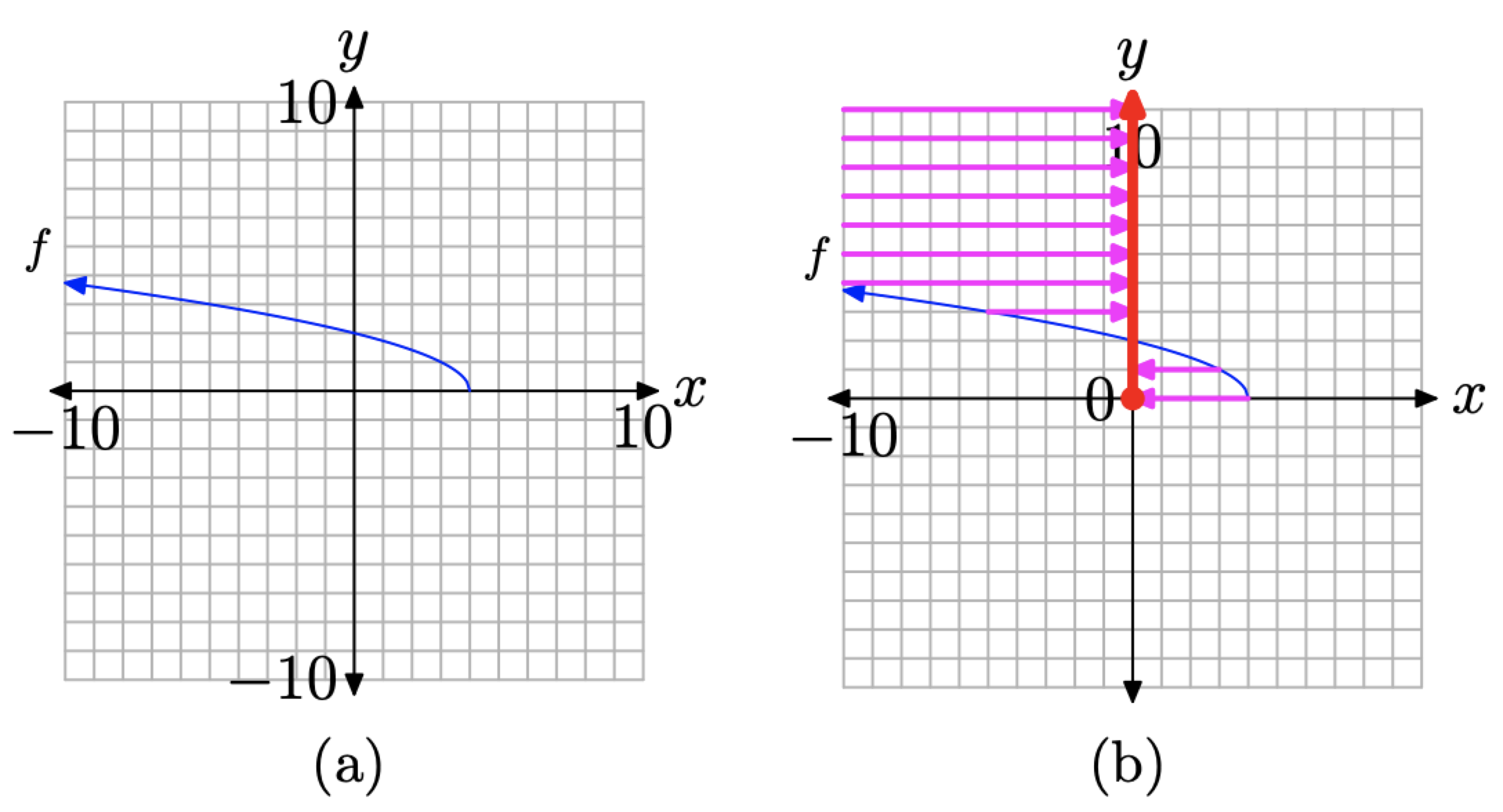
Figure 4.3.16. Determining the range of f(x)=√4−x from its graph.
2. Again, we assume that the right end of the graph of f ends at the point (4,0). The projection of this point onto the y-axis produces the “filled” endpoint at the origin shown in Figure 4.3.16(b).
Note that the “shadow” or projection onto the y-axis in Figure 4.3.16(b) includes all values of y that are greater than or equal to zero. Hence,
Range of f=[0,∞)={y:y≥0}