3.5: Absolute Value Functions

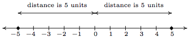
There are a few ways to describe what is meant by the absolute value \(|x|\) of a real number \(x\). You may have been taught that \(|x|\) is the distance from the real number \(x\) to \(0\) on the number line. So, for example, \(|5| = 5\) and \(|-5| = 5\), since each is \(5\) units from \(0\) on the number line.

Another way to define absolute value is by the equation \(|x| = \sqrt{x^2}\). Using this definition, we have \(|5| = \sqrt{(5)^2} = \sqrt{25} = 5\) and \(|-5| = \sqrt{(-5)^2} = \sqrt{25} = 5\). The long and short of both of these procedures is that \(|x|\) takes negative real numbers and assigns them to their positive counterparts while it leaves positive numbers alone. This last description is the one we shall adopt, and is summarized in the following definition.

Definition 2.4: Absolute Value

The absolute value of a real number \(x\), denoted \(|x|\), is given by

\[ |x| = \left\{ \begin{array}{rcl} -x, & \mbox{if} & x < 0 \\ x, & \mbox{if} & x \geq 0 \\ \end{array} \right. \label{absolutevalue}\]

In Definition 2.4, we define \(|x|\) using a piecewise-defined function (Section 1.4). To check that this definition agrees with what we previously understood as absolute value, note that since \(5 \geq 0\), to find \(|5|\) we use the rule \(|x| = x\), so \(|5|=5\). Similarly, since \(-5 < 0\), we use the rule \(|x| = -x\), so that \(|-5| = -(-5) = 5\). This is one of the times when it's best to interpret the expression '\(-x\)' as 'the opposite of \(x\)' as opposed to 'negative \(x\)'. Before we begin studying absolute value functions, we remind ourselves of the properties of absolute value.

Theorem 2.1: Properties of Absolute Value

Let \(a\), \(b\) and \(x\) be real numbers and let \(n\) be an integer, then:

• Product Rule: \(|ab|= |a||b|\)
• Power Rule: \(\left| a^{n} \right| = |a|^{n}\) whenever \(a^{n}\) is defined
• Quotient Rule: \(\left| \dfrac{a}{b} \right| = \dfrac{|a|}{|b|}\), provided \(b \neq 0\)

Equality Properties:

• \(|x| = 0\) if and only if \(x = 0\).
• For \(c > 0\), \(|x| = c\) if and only if \(x = c\) or \(x = -c\).
• For \(c < 0\), \(|x| = c\) has no solution.

The proofs of the Product and Quotient Rules in Theorem 2.1 boil down to checking four cases:

• when both \(a\) and \(b\) are positive;
• when they are both negative;
• when one is positive and the other is negative;
• and when one or both are zero.

For example, suppose we wish to show that \(|ab| = |a||b|\). We need to show that this equation is true for all real numbers \(a\) and \(b\). If \(a\) and \(b\) are both positive, then so is \(ab\). Hence, \(|a| = a\), \(|b| = b\) and \(|ab| = ab\). Hence, the equation \(|ab| = |a||b|\) is the same as \(ab = ab\) which is true. If both \(a\) and \(b\) are negative, then \(ab\) is positive. Hence, \(|a| = -a\), \(|b| = -b\) and \(|ab| = ab\). The equation \(|ab| = |a||b|\) becomes \(ab = (-a)(-b)\), which is true. Suppose \(a\) is positive and \(b\) is negative. Then \(ab\) is negative, and we have \(|ab| = -ab\), \(|a| = a\) and \(|b| = -b\). The equation \(|ab| = |a||b|\) reduces to \(-ab = a(-b)\) which is true. A symmetric argument shows the equation \(|ab| = |a||b|\) holds when \(a\) is negative and \(b\) is positive. Finally, if either \(a\) or \(b\) (or both) are zero, then both sides of \(|ab| = |a||b|\) are zero, so the equation holds in this case, too. All of this rhetoric has shown that the equation \(|ab| = |a||b|\) holds true in all cases.

The proof of the Quotient Rule is very similar, with the exception that \(b \neq 0\). The Power Rule can be shown by repeated application of the Product Rule. The 'Equality Properties' can be proved using Definition 2.4 and by looking at the cases when \(x\geq 0\), in which case \(|x| = x\), or when \(x<0\), in which case \(|x| = -x\). For example, if \(c>0\), and \(|x| = c\), then if \(x \geq 0\), we have \(x = |x| = c\). If, on the other hand, \(x < 0\), then \(-x = |x| = c\), so \(x = -c\). The remaining properties are proved similarly and are left for the Exercises. Our first example reviews how to solve basic equations involving absolute value using the properties listed in Theorem 2.1.

Example \(\PageIndex{1}\): Absolute Value

Solve each of the following equations.

1. \(|3x-1| = 6\)
2. \(3 - |x+5| = 1\)
3. \(3|2x+1| - 5 = 0\)
4. \(4 - |5x+3| = 5\)
5. \(|x| = x^2-6\)
6. \(|x-2| + 1 = x\)

Solution

1. The equation \(|3x-1| = 6\) is of the form \(|x| = c\) for \(c>0\), so by the Equality Properties, \(|3x-1| = 6\) is equivalent to \(3x-1=6\) or \(3x-1 = -6\). Solving the former, we arrive at \(x = \frac{7}{3}\), and solving the latter, we get \(x = -\frac{5}{3}\). We may check both of these solutions by substituting them into the original equation and showing that the arithmetic works out.

To use the Equality Properties to solve \(3 - |x+5| = 1\), we first isolate the absolute value.

\[ \begin{array}{rclr} 3 - |x+5| & = & 1 & \\ -|x+5| & = & -2 & \text{subtract \(3\)} \\ |x+5| & = & 2 & \text{divide by \(-1\)} \\ \end{array} \]

From the Equality Properties, we have \(x+5 = 2\) or \(x+5 = -2\), and get our solutions to be \(x = -3\) or \(x = -7\). We leave it to the reader to check both answers in the original equation.

1. As in the previous example, we first isolate the absolute value in the equation \(3|2x+1| - 5 = 0\) and get \(|2x+1| = \frac{5}{3}\). Using the Equality Properties, we have \(2x+1 = \frac{5}{3}\) or \(2x+1 = -\frac{5}{3}\). Solving the former gives \(x = \frac{1}{3}\) and solving the latter gives \(x = -\frac{4}{3}\). As usual, we may substitute both answers in the original equation to check.
2. Upon isolating the absolute value in the equation \(4 - |5x+3| = 5\), we get \(|5x+3| = -1\). At this point, we know there cannot be any real solution, since, by definition, the absolute value of anything is never negative. We are done.
3. The equation \(|x| = x^2-6\) presents us with some difficulty, since \(x\) appears both inside and outside of the absolute value. Moreover, there are values of \(x\) for which \(x^2-6\) is positive, negative and zero, so we cannot use the Equality Properties without the risk of introducing extraneous solutions, or worse, losing solutions. For this reason, we break equations like this into cases by rewriting the term in absolute values, \(|x|\), using Definition 2.4. For \(x < 0\), \(|x| = -x\), so for \(x < 0\), the equation \(|x| = x^2-6\) is equivalent to \(-x = x^2-6\). Rearranging this gives us \(x^2+x-6 = 0\), or \((x+3)(x-2) = 0\). We get \(x = -3\) or \(x=2\). Since only \(x=-3\) satisfies \(x<0\), this is the answer we keep. For \(x \geq 0\), \(|x| = x\), so the equation \(|x| = x^2-6\) becomes \(x = x^2-6\). From this, we get \(x^2-x-6 =0\) or \((x-3)(x+2) = 0\). Our solutions are \(x=3\) or \(x = -2\), and since only \(x=3\) satisfies \(x \geq 0\), this is the one we keep. Hence, our two solutions to \(|x| = x^2-6\) are \(x=-3\) and \(x=3\).
4. To solve \(|x-2| + 1 = x\), we first isolate the absolute value and get \(|x-2| = x-1\). Since we see \(x\) both inside and outside of the absolute value, we break the equation into cases. The term with absolute values here is \(|x-2|\), so we replace '\(x\)' with the quantity '\((x-2)\)' in Definition 2.4 to get \[ |x-2| = \left\{ \begin{array}{rcl} -(x-2), & \mbox{if} & (x-2) < 0 \\ (x-2), & \mbox{if} & (x-2) \geq 0 \\ \end{array} \right.\]

Simplifying yields \[ |x-2| = \left\{ \begin{array}{rcl} -x+2, & \mbox{if} & x < 2 \\ x-2, & \mbox{if} & x \geq 2 \\ \end{array} \right.\]

So, for \(x<2\), \(|x-2| = -x+2\) and our equation \(|x-2| = x-1\) becomes \(-x+2 = x-1\), which gives \(x = \frac{3}{2}\). Since this solution satisfies \(x < 2\), we keep it. Next, for \(x \geq 2\), \(|x-2| = x-2\), so the equation \(|x-2| = x-1\) becomes \(x-2 = x-1\). Here, the equation reduces to \(-2 = -1\), which signifies we have no solutions here. Hence, our only solution is \(x = \frac{3}{2}\).

Next, we turn our attention to graphing absolute value functions. Our strategy in the next example is to make liberal use of Definition 2.4 along with what we know about graphing linear functions (from Section 2.1 ) and piecewise-defined functions (from Section 1.4).

Example \(\PageIndex{2}\):

Graph each of the following functions.

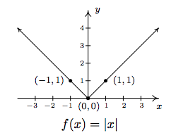
1. \(f(x) = |x|\)
2. \(g(x) = |x-3|\)
3. \(h(x) = |x| -3\)
4. \(i(x) = 4 - 2|3x+1|\)

Find the zeros of each function and the \(x\)- and \(y\)-intercepts of each graph, if any exist. From the graph, determine the domain and range of each function, list the intervals on which the function is increasing, decreasing or constant, and find the relative and absolute extrema, if they exist.

Solution

1. To find the zeros of \(f\), we set \(f(x)= 0\). We get \(|x|=0\), which, by Theorem \(\PageIndex{1}\) gives us \(x=0\). Since the zeros of \(f\) are the \(x\)-coordinates of the \(x\)-intercepts of the graph of \(y=f(x)\), we get \((0,0)\) as our only \(x\)-intercept. To find the \(y\)-intercept, we set \(x=0\), and find \(y = f(0) = 0\), so that \((0,0)\) is our \(y\)-intercept as well.\footnote{Actually, since functions can have at most one \(y\)-intercept (Do you know why?), as soon as we found \((0,0)\) as the \(x\)-intercept, we knew this was also the \(y\)-intercept.} Using Definition \(\PageIndex{1}\), we get \[ f(x) = |x| = \left\{ \begin{array}{rcl} -x, & \mbox{if} & x < 0 \\ x, & \mbox{if} & x \geq 0 \\ \end{array} \right.\] Hence, for \(x < 0\), we are graphing the line \(y = -x\); for \(x \geq 0\), we have the line \(y = x\). Proceeding as we did in Section 1.6, we get

Notice that we have an 'open circle' at \((0,0)\) in the graph when \(x<0\). As we have seen before, this is due to the fact that the points on \(y = -x\) approach \((0,0)\) as the \(x\)-values approach \(0\). Since \(x\) is required to be strictly less than zero on this stretch, the open circle is drawn at the origin. However, notice that when \(x \geq 0\), we get to fill in the point at \((0,0)\), which effectively 'plugs' the hole indicated by the open circle. Thus we get,

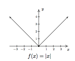
By projecting the graph to the \(x\)-axis, we see that the domain is \((-\infty, \infty)\). Projecting to the \(y\)-axis gives us the range \([0,\infty)\). The function is increasing on \([0,\infty)\) and decreasing on \((-\infty,0]\). The relative minimum value of \(f\) is the same as the absolute minimum, namely \(0\) which occurs at \((0,0)\). There is no relative maximum value of \(f\). There is also no absolute maximum value of \(f\), since the \(y\) values on the graph extend infinitely upwards.

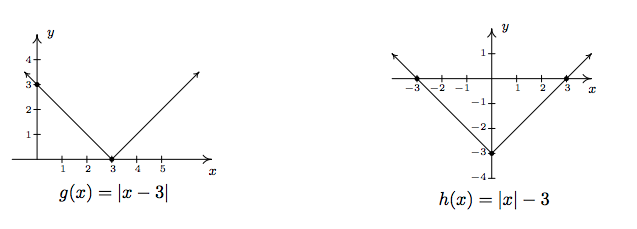
2. To find the zeros of \(g\), we set \(g(x) = |x-3|=0\). By Theorem 2.1, we get \(x-3=0\) so that \(x=3\). Hence, the \(x\)-intercept is \((3,0)\). To find our \(y\)-intercept, we set \(x=0\) so that \(y = g(0) = |0-3| = 3\), which yields \((0,3)\) as our \(y\)-intercept. To graph \(g(x) = |x-3|\), we use Definition 2.4 to rewrite \(g\) as

\[ g(x) = |x-3| = \left\{ \begin{array}{rcl} -(x-3), & \mbox{if} & (x-3) < 0 \\ (x-3), & \mbox{if} & (x -3) \geq 0 \\ \end{array} \right.\]

Simplifying, we get

\[ g(x) =\left\{ \begin{array}{rcl} -x+3, & \mbox{if} & x<3 \\ x-3, & \mbox{if} & x \geq 3 \\ \end{array} \right.\]

As before, the open circle we introduce at \((3,0)\) from the graph of \(y = -x+3\) is filled by the point \((3,0)\) from the line \(y = x-3\). We determine the domain as \((-\infty, \infty)\) and the range as \([0,\infty)\). The function \(g\) is increasing on \([3,\infty)\) and decreasing on \((-\infty,3]\). The relative and absolute minimum value of \(g\) is \(0\) which occurs at \((3,0)\). As before, there is no relative or absolute maximum value of \(g\).

3. Setting \(h(x) = 0\) to look for zeros gives \(|x|-3=0\). As in Example \(\PageIndex{1}\), we isolate the absolutre value to get \(|x| = 3\) so that \(x =3\) or \(x=-3\). As a result, we have a pair of \(x\)-intercepts: \((-3,0)\) and \((3,0)\). Setting \(x=0\) gives \(y = h(0) = |0|-3 = -3\), so our \(y\)-intercept is \((0,-3)\). As before, we rewrite the absolute value in \(h\) to get

\[ h(x) =\left\{ \begin{array}{rcl} -x-3, & \mbox{if} & x<0 \\ x-3, & \mbox{if} & x \geq 0 \\ \end{array} \right.\]

Once again, the open circle at \((0,-3)\) from one piece of the graph of \(h\) is filled by the point \((0,-3)\) from the other piece of \(h\). From the graph, we determine the domain of \(h\) is \((-\infty, \infty)\) and the range is \([-3,\infty)\). On \([0,\infty)\), \(h\) is increasing; on \((-\infty,0]\) it is decreasing. The relative minimum occurs at the point \((0,-3)\) on the graph, and we see \(-3\) is both the relative and absolute minimum value of \(h\). Also, \(h\) has no relative or absolute maximum value.

4. As before, we set \(i(x)=0\) to find the zeros of \(i\) and get \(4 - 2|3x+1|=0\). Isolating the absolute value term gives \(|3x+1|=2\), so either \(3x+1 = 2\) or \(3x+1=-2\). We get \(x=\frac{1}{3}\) or \(x=-1\), so our \(x\)-intercepts are \(\left(\frac{1}{3},0\right)\) and \((-1,0)\). Substituting \(x=0\) gives \(y = i(0) = 4-2|3(0)+1| = 2\), for a \(y\)-intercept of \((0,2)\). Rewriting the formula for \(i(x)\) without absolute values gives

\[ i(x) =\left\{ \begin{array}{rcl} 4-2(-(3x+1)), & \mbox{if} & (3x+1) <0 \\ 4-2(3x+1), & \mbox{if} & (3x+1) \geq 0 \\ \end{array} \right. = \left\{ \begin{array}{rcl} 6x+6, & \mbox{if} & x < -\frac{1}{3} \\[2pt] -6x+2, & \mbox{if} & x \geq - \frac{1}{3} \\ \end{array} \right. \]

The usual analysis near the trouble spot \(x=-\frac{1}{3}\) gives the 'corner' of this graph is \(\left( -\frac{1}{3}, 4\right)\), and we get the distinctive '\(\vee\)' shape:

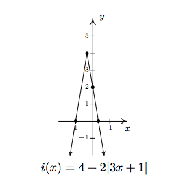
The domain of \(i\) is \((-\infty, \infty)\) while the range is \((-\infty, 4]\). The function \(i\) is increasing on \(\left(-\infty, -\frac{1}{3}\right]\) and decreasing on \(\left[ -\frac{1}{3}, \infty\right)\). The relative maximum occurs at the point \(\left(-\frac{1}{3}, 4\right)\) and the relative and absolute maximum value of \(i\) is \(4\). Since the graph of \(i\) extends downwards forever more, there is no absolute minimum value. As we can see from the graph, there is no relative minimum, either.

Note that all of the functions in the previous example bear the characteristic '\(\vee\)' shape of the graph of \(y=|x|\). We could have graphed the functions \(g\), \(h\) and \(i\) in Example \(\PageIndex{2}\) starting with the graph of \(f(x)=|x|\) and applying transformations as in Section 1.7 as our next example illustrates.

Example \(\PageIndex{3}\):

Graph the following functions starting with the graph of \(f(x) = |x|\) and using transformations.

1. \(g(x) = |x-3|\)
2. \(h(x) = |x| - 3\)
3. \(i(x) = 4-2|3x+1|\)

Solution

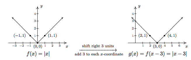
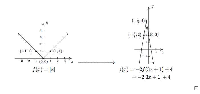
We begin by graphing \(f(x) = |x|\) and labeling three points, \((-1,1)\), \((0,0)\) and \((1,1)\).

1. Since \(g(x) = |x-3| = f(x-3)\), Theorem 1.7 tells us to add \(3\) to each of the \(x\)-values of the points on the graph of \(y=f(x)\) to obtain the graph of \(y=g(x)\). This shifts the graph of \(y=f(x)\) to the right \(3\) units and moves the point \((-1,1)\) to \((2,1)\), \((0,0)\) to \((3,0)\) and \((1,1)\) to \((4,1)\). Connecting these points in the classic '\(\vee\)' fashion produces the graph of \(y = g(x)\).

2. For \(h(x) = |x| - 3 = f(x) -3\), Theorem 1.7 tells us to subtract \(3\) from each of the \(y\)-values of the points on the graph of \(y=f(x)\) to obtain the graph of \(y = h(x)\). This shifts the graph of \(y=f(x)\) down \(3\) units and moves \((-1,1)\) to \((-1,-2)\), \((0,0)\) to \((0,-3)\) and \((1,1)\) to \((1,-2)\). Connecting these points with the '\(\vee\)' shape produces our graph of \(y=h(x)\).

3. We re-write \(i(x) = 4-2|3x+1| = 4-2f(3x+1) = -2f(3x+1) + 4\) and apply Theorem 1.7. First, we take care of the changes on the 'inside' of the absolute value. Instead of \(|x|\), we have \(|3x+1|\), so, in accordance with Theorem 1.7, we first subtract \(1\) from each of the \(x\)-values of points on the graph of \(y = f(x)\), then divide each of those new values by \(3\). This effects a horizontal shift left \(1\) unit followed by a horizontal shrink by a factor of \(3\). These transformations move \((-1,1)\) to \(\left(-\frac{2}{3}, 1 \right)\), \((0,0)\) to \(\left(-\frac{1}{3}, 0 \right)\) and \((1,1)\) to \(\left(0,1\right)\). Next, we take care of what's happening 'outside of' the absolute value. Theorem 1.7 instructs us to first multiply each \(y\)-value of these new points by \(-2\) then add \(4\). Geometrically, this corresponds to a vertical stretch by a factor of \(2\), a reflection across the \(x\)-axis and finally, a vertical shift up \(4\) units. These transformations move \(\left(-\frac{2}{3}, 1 \right)\) to \(\left(-\frac{2}{3}, 2 \right)\), \(\left(-\frac{1}{3}, 0 \right)\) to \(\left(-\frac{1}{3}, 4 \right)\), and \(\left(0,1\right)\) to \(\left(0, 2\right)\). Connecting these points with the usual '\(\vee\)' shape produces our graph of \(y = i(x)\).

While the methods in Section 1.7 can be used to graph an entire family of absolute value functions, not all functions involving absolute values posses the characteristic '\(\vee\)' shape. As the next example illustrates, often there is no substitute for appealing directly to the definition.

Example \(\PageIndex{4}\):

Graph each of the following functions. Find the zeros of each function and the \(x\)- and \(y\)-intercepts of each graph, if any exist. From the graph, determine the domain and range of each function, list the intervals on which the function is increasing, decreasing or constant, and find the relative and absolute extrema, if they exist.

1. \(f(x) = \dfrac{|x|}{x}\)
2. \(g(x) = |x+2| - |x-3|+1\)

Solution

1. We first note that, due to the fraction in the formula of \(f(x)\), \(x \neq 0\). Thus the domain is \((-\infty, 0) \cup (0, \infty)\). To find the zeros of \(f\), we set \(f(x) = \frac{|x|}{x} = 0\). This last equation implies \(|x|=0\), which, from Theorem \(\PageIndex{1}\), implies \(x=0\). However, \(x=0\) is not in the domain of \(f\), which means we have, in fact, no \(x\)-intercepts. We have no \(y\)-intercepts either, since \(f(0)\) is undefined. Re-writing the absolute value in the function gives

\[ f(x) =\left\{ \begin{array}{rcl} \dfrac{-x}{x}, & \mbox{if} & x <0 \\ [10pt] \dfrac{x}{x}, & \mbox{if} & x > 0 \\ \end{array} \right. = \left\{ \begin{array}{rcl} -1, & \mbox{if} & x < 0 \\ 1, & \mbox{if} & x >0 \\ \end{array} \right. \]

To graph this function, we graph two horizontal lines: \(y = -1\) for \(x < 0\) and \(y = 1\) for \(x > 0\). We have open circles at \((0,-1)\) and \((0,1)\) (Can you explain why?) so we get

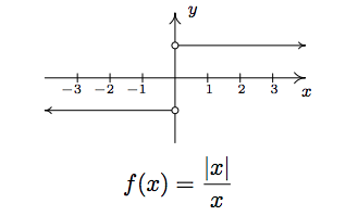
As we found earlier, the domain is \((-\infty, 0)\cup(0,\infty)\). The range consists of just two \(y\)-values: \(\{-1,1\}\). The function \(f\) is constant on \((-\infty,0)\) and \((0,\infty)\). The local minimum value of \(f\) is the absolute minimum value of \(f\), namely \(-1\); the local maximum and absolute maximum values for \(f\) also coincide \(-\) they both are \(1\). Every point on the graph of \(f\) is simultaneously a relative maximum and a relative minimum. (Can you remember why in light of Definition 1.11? This was explored in the Exercises in Section 1.6 .)

2. To find the zeros of \(g\), we set \(g(x) = 0\). The result is \(|x+2|-|x-3| +1 = 0\). Attempting to isolate the absolute value term is complicated by the fact that there are \textbf{two} terms with absolute values. In this case, it easier to proceed using cases by re-writing the function \(g\) with two separate applications of Definition 2.4 to remove each instance of the absolute values, one at a time. In the first round we get

\[ g(x) =\left\{ \begin{array}{rcl} -(x+2) - |x-3|+1, & \mbox{if} & (x+2) <0 \\ (x+2) - |x-3|+1, & \mbox{if} & (x+2) \geq 0 \\ \end{array} \right. = \left\{ \begin{array}{rcl} -x-1 - |x-3|, & \mbox{if} & x<-2 \\ x+3-|x-3|, & \mbox{if} & x \geq -2 \\ \end{array} \right. \]

Given that

\[ |x-3| =\left\{ \begin{array}{rcl} -(x-3), & \mbox{if} & (x-3) <0 \\ x-3, & \mbox{if} & (x-3) \geq 0 \\ \end{array} \right. = \left\{ \begin{array}{rcl} -x+3, & \mbox{if} & x<3 \\ x-3, & \mbox{if} & x \geq 3 \\ \end{array} \right., \]

we need to break up the domain again at \(x=3\). Note that if \(x < -2\), then \(x < 3\), so we replace \(|x-3|\) with \(-x+3\) for that part of the domain, too. Our completed revision of the form of \(g\) yields

\[ g(x) = \left\{ \begin{array}{rcl} -x-1 - (-x+3), & \mbox{if} & x<-2 \\ x+3-(-x+3), & \mbox{if} & x \geq -2 \, \mbox{ and } \, x < 3 \\ x+3 - (x-3), & \mbox{if} & x \geq 3 \\ \end{array} \right. \;\; = \;\; \left\{ \begin{array}{rcl} -4, & \mbox{if} & x<-2 \\ 2x, & \mbox{if} & -2 \leq x < 3 \\ 6, & \mbox{if} & x \geq 3 \\ \end{array} \right. \]

To solve \(g(x)=0\), we see that the only piece which contains a variable is \(g(x) = 2x\) for \(-2 \leq x < 3\). Solving \(2x=0\) gives \(x=0\). Since \(x=0\) is in the interval \([-2,3)\), we keep this solution and have \((0,0)\) as our only \(x\)-intercept. Accordingly, the \(y\)-intercept is also \((0,0)\). To graph \(g\), we start with \(x < -2\) and graph the horizontal line \(y=-4\) with an open circle at \((-2,-4)\). For \(-2 \leq x < 3\), we graph the line \(y=2x\) and the point \((-2,-4)\) patches the hole left by the previous piece. An open circle at \((3,6)\) completes the graph of this part. Finally, we graph the horizontal line \(y=6\) for \(x \geq 3\), and the point \((3,6)\) fills in the open circle left by the previous part of the graph. The finished graph is

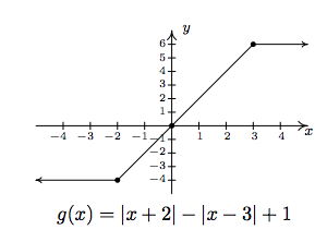
The domain of \(g\) is all real numbers, \((-\infty, \infty)\), and the range of \(g\) is all real numbers between \(-4\) and \(6\) inclusive, \([-4,6]\). The function is increasing on \([-2,3]\) and constant on \((-\infty, -2]\) and \([3,\infty)\). The relative minimum value of \(f\) is \(-4\) which matches the absolute minimum. The relative and absolute maximum values also coincide at \(6\). Every point on the graph of \(y=g(x)\) for \(x<-2\) and \(x> 3\) yields both a relative minimum and relative maximum. The point \((-2,-4)\), however, gives only a relative minimum and the point \((3,6)\) yields only a relative maximum. (Recall the Exercises in Section 1.6 which dealt with constant functions.)

Many of the applications that the authors are aware of involving absolute values also involve absolute value inequalities. For that reason, we save our discussion of applications for Section 2.4.