1.3: Rates of Change and Behavior of Graphs

Since functions represent how an output quantity varies with an input quantity, it is natural to ask about the rate at which the values of the function are changing. For example, the function \(C(t)\) below gives the average cost, in dollars, of a gallon of gasoline \(t\) years after 2000.

\(t\)	2	3	4	5	6	7	8	9
\(C(t)\)	1.47	1.69	1.94	2.30	2.51	2.64	3.01	2.14

If we were interested in how the gas prices had changed between 2002 and 2009, we could compute that the cost per gallon had increased from $1.47 to $2.14, an increase of $0.67. While this is interesting, it might be more useful to look at how much the price changed per year. You are probably noticing that the price didn’t change the same amount each year, so we would be finding the average rate of change over a specified amount of time.

The gas price increased by $0.67 from 2002 to 2009, over 7 years, for an average of \(\dfrac{\$ 0.67}{7years} \approx 0.096\)dollars per year. On average, the price of gas increased by about 9.6 cents each year.

Definition: Rate of Change

A rate of change describes how the output quantity changes in relation to the input quantity. The units on a rate of change are output units per input units.

Some other examples of rates of change would be quantities like:

• A population of rats increases by 40 rats per week
• A barista earns $9 per hour (dollars per hour)
• A farmer plants 60,000 onions per acre
• A car can drive 27 miles per gallon
• A population of grey whales decreases by 8 whales per year
• The amount of money in your college account decreases by $4,000 per quarter

Definition: Average Rate of Change

The average rate of change between two input values is the total change of the function values (output values) divided by the change in the input values.

\[\text{Average rate of change} = \dfrac{\text{Change of Output}}{\text{Change of Input}} = \dfrac{\Delta y}{\Delta x} =\dfrac{y_{2} -y_{1} }{x_{2} -x_{1} }\]

Example \(\PageIndex{1}\)

Using the cost-of-gas function from earlier, find the average rate of change between 2007 and 2009.

Solution

From the table, in 2007 the cost of gas was $2.64. In 2009 the cost was $2.14.

The input (years) has changed by 2. The output has changed by $2.14 - $2.64 = -0.50.

The average rate of change is then \(\dfrac{-\$ 0.50}{2years}\) = -0.25 dollars per year

Exercise \(\PageIndex{1}\)

Using the same cost-of-gas function, find the average rate of change between 2003 and 2008

Answer

\(\dfrac{$3.01 - $1.69}{5\ years} = \dfrac{$1.32}{5\ years} = 0.264\) dollars per year.

Notice that in the last example the change of output was negative since the output value of the function had decreased. Correspondingly, the average rate of change is negative.

Example \(\PageIndex{2}\)

Given the function \(g(t)\) shown here, find the average rate of change on the interval [0, 3].

Solution

At t = 0, the graph shows \(g(0) = 1\)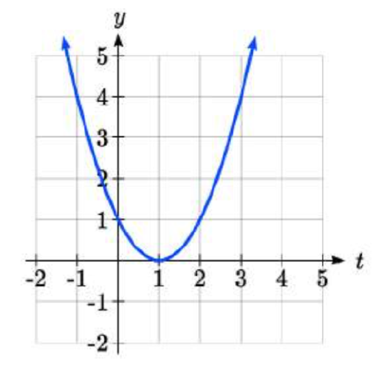

At t = 3, the graph shows \(g(3) = 4\)

The output has changed by 3 while the input has changed by 3, giving an average rate of change of:

\[\dfrac{4-1}{3-0} =\dfrac{3}{3} =1\nonumber \]

Example \(\PageIndex{3}\)

On a road trip, after picking up your friend who lives 10 miles away, you decide to record your distance from home over time. Find your average speed over the first 6 hours.

\(t\) (hours)	0	1	2	3	4	5	6	7
\(D(t)\) (miles)	10	55	90	153	214	240	292	300

Solution

Here, your average speed is the average rate of change.

You traveled 282 miles in 6 hours, for an average speed of

\[\dfrac{292-10}{6-0} =\dfrac{282}{6}= 47\text{ miles per hour}\nonumber\]

We can more formally state the average rate of change calculation using function notation.

Definition: Average Rate of Change using Function Notation

Given a function \(f(x)\), the average rate of change on the interval [a, b] is

\[\text{Average rate of change} = \dfrac{\text{Change of Output}}{\text{Change of Input}} =\dfrac{f(b)-f(a)}{b-a} \label{avgratefunction}\]

Example \(\PageIndex{4}\)

Compute the average rate of change of \(f(x)=x^{2} -\dfrac{1}{x}\) on the interval [2, 4].

Solution

We can start by computing the function values at each endpoint of the interval

\[f(2)=2^{2} -\dfrac{1}{2} =4-\dfrac{1}{2} =\dfrac{7}{2} \nonumber\]

\[f(4)=4^{2} -\dfrac{1}{4} =16-\dfrac{1}{4} =\dfrac{63}{4} \nonumber\]

Now computing the average rate of change

\[\text{Average rate of change} = \dfrac{f(4) - f(2)}{4 - 2} =\dfrac{\dfrac{63}{4} -\dfrac{7}{2} }{4-2} =\dfrac{\dfrac{49}{4} }{2} = \dfrac{49}{8} \nonumber\]

Exercise \(\PageIndex{2}\)

Find the average rate of change of \(f(x) = x - 2\sqrt{x}\) on the interval [1, 9].

Answer

Average rate of change = \(\dfrac{f(9) - f(1)}{9 - 1} = \dfrac{(9 - 2\sqrt{9}) - (1 - 2\sqrt{1})}{9 - 1} = \dfrac{(3) - (-1)}{9 - 1} = \dfrac{4}{8} = \dfrac{1}{2}\)

Example \(\PageIndex{5}\)

The magnetic force \(F\), measured in Newtons, between two magnets is related to the distance between the magnets \(d\), in centimeters, by the formula \(F(d)=\dfrac{2}{d^{2} }\). Find the average rate of change of force if the distance between the magnets is increased from 2 cm to 6 cm.

Solution

We are computing the average rate of change of \(F(d)=\dfrac{2}{d^{2} }\) on the interval [2, 6].

Average rate of change = \(\dfrac{F(6) - F(2)}{6 - 2}\)

Evaluating the function

\[\dfrac{F(6)-F(2)}{6-2} =\nonumber \]

\[= \dfrac{\dfrac{2}{6^{2} } -\dfrac{2}{2^{2} } }{6-2}\nonumber \] Simplifying

\[= \dfrac{\dfrac{2}{36} -\dfrac{2}{4} }{4}\nonumber \] Combining the numerator terms

\[= \dfrac{\dfrac{-16}{36} }{4}\nonumber \] Simplifying further

\[= \dfrac{-1}{9}\nonumber \] Newtons per centimeter

This tells us the magnetic force decreases, on average, by 1/9 Newtons per centimeter over this interval.

Example \(\PageIndex{6}\)

Find the average rate of change of \(g(t)=t^{2} +3t+1\)on the interval \([0, a]\). Your answer will be an expression involving a.

Solution

Using the average rate of change formula

\[\dfrac{g(a)-g(0)}{a-0}\nonumber\]

Evaluating the function

\[\dfrac{(a^{2} +3a+1)-(0^{2} +3(0)+1)}{a-0}\nonumber\]

Simplifying

\[\dfrac{a^{2} +3a+1-1}{a}\nonumber\]

Simplifying further, and factoring

\[\dfrac{a(a+3)}{a}\nonumber\]

Cancelling the common factor \(a\)

\[a+3\nonumber\]

This result tells us the average rate of change between t = 0 and any other point t = a. For example, on the interval [0, 5], the average rate of change would be 5+3 = 8.

Exercise \(\PageIndex{3}\)

Find the average rate of change of \(f(x)=x^{3} +2\) on the interval \([a,a+h]\).

Answer

\[\dfrac{f(a + h) - f(a)}{(a + h) - a} = \dfrac{((a + h)^3 + 2) - (a^3 + 2)}{h} = \dfrac{a^3 + 3a^2h + 3ah^2 + h^3 + 2 - a^3 - 2}{h} = \dfrac{3a^2h + 3ah^2 + h^3}{h} = \dfrac{h(3a^2 + 3ah + h^2)}{h} = 3a^2 + 3ah + h^2\nonumber\]

Application to Business

In business, average rate of change is related to the idea of marginal cost, marginal revenue, and marginal profit.

Definition: Marginal Cost/Revenue/Profit

Marginal Cost is typically defined as the change in total cost if the quantity of items produced increases by one.  Likewise, marginal revenue and marginal profit are the change in revenue and profit if the quantity of items increases by one.

In practice, marginal cost is usually calculated another way, using calculus techniques you will learn in future courses.  In this course, though, we will stick with calculating marginal cost by looking at the actual change of total cost when production increases by one.

Example \(\PageIndex{7}\)

A company has determined the total cost of producing \(q\)  items is \(TC(q) = 2000 + 50\sqrt{q}\).  Find the marginal cost, when production is currently 5000 items.

Solution

We want to find the increase in total cost when increasing production from 5000 items to 5001 items.  This is equivalent to finding the average rate of change on the interval \([5000, 5001]\).

The total cost at 5000 items is:  \(TC(5000) = 2000 + 50\sqrt {5000}  \approx 5535.53\)

The total cost at 5001 items is:  \(TC(5001) = 2000 + 50\sqrt {5001}  \approx 5535.89\)

 

The marginal cost is \(5535.89 – 5535.53 = \$0.36\).

 

In other words, after producing 5000 items, the additional cost of producing the 5001^st item is $0.36

Graphical Behavior of Functions

As part of exploring how functions change, it is interesting to explore the graphical behavior of functions.

Definition: increasing/decreasing

A function is increasing on an interval if the function values increase as the inputs increase. More formally, a function is increasing if \(f(b) > f(a)\) for any two input values a and b in the interval with \(b > a\). The average rate of change of an increasing function is positive.

A function is decreasing on an interval if the function values decrease as the inputs increase. More formally, a function is decreasing if \(f(b) < f(a)\) for any two input values a and b in the interval with \(b > a\). The average rate of change of a decreasing function is negative.

Example \(\PageIndex{8}\)

Given the function \(p(t)\) graphed here, on what intervals does the function appear to be increasing?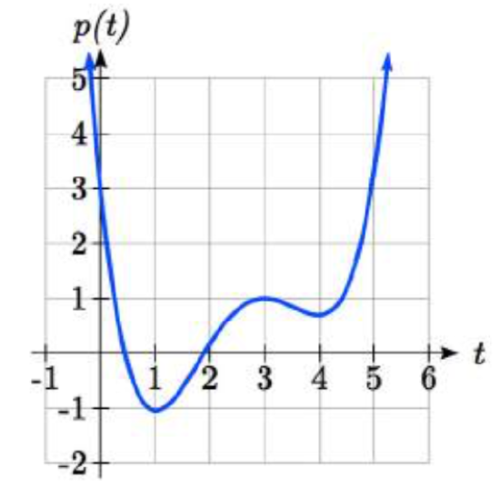

The function appears to be increasing from \(t = 1\) to \(t = 3\), and from \(t = 4\) on.

In interval notation, we would say the function appears to be increasing on the interval \((1, 3)\)and the interval \((4, \infty)\).

Solution

Add text here.

Notice in the last example that we used open intervals (intervals that don’t include the endpoints) since the function is neither increasing nor decreasing at \(t =\) 1, 3, or 4.

Definition: Local Extrema

A point where a function changes from increasing to decreasing is called a local maximum.

A point where a function changes from decreasing to increasing is called a local minimum.

Together, local maxima and minima are called the local extrema, or local extreme values, of the function.

Example \(\PageIndex{9}\)

Using the cost of gasoline function from the beginning of the section, find an interval on which the function appears to be decreasing. Estimate any local extrema using the table.

\(t\)	2	3	4	5	6	7	8	9
\(C(t)\)	1.47	1.69	1.94	2.30	2.51	2.64	3.01	2.14

It appears that the cost of gas increased from \(t = 2\) to \(t = 8\). It appears the cost of gas decreased from \(t = 8\) to \(t = 9\), so the function appears to be decreasing on the interval (8, 9).

Since the function appears to change from increasing to decreasing at \(t = 8\), there is local maximum at \(t = 8\).

Example \(\PageIndex{10}\)

Use a graph to estimate the local extrema of the function \(f(x)=\dfrac{2}{x} +\dfrac{x}{3}\). Use these to determine the intervals on which the function is increasing.

Solution

Using technology to graph the function, it appears there is a local minimum somewhere between \(x = 2\) and \(x = 3\), and a symmetric local maximum somewhere between \(x = -3\) and \(x = -2\).

Most graphing calculators and graphing utilities can estimate the location of maxima and minima. Below are screen images from two different technologies, showing the estimate for the local maximum and minimum.

Based on these estimates, the function is increasing on the intervals \((-\infty , -2.449)\)and \((2.449, \infty )\). Notice that while we expect the extrema to be symmetric, the two different technologies agree only up to 4 decimals due to the differing approximation algorithms used by each.

Exercise \(\PageIndex{4}\)

Use a graph of the function \(f(x)=x^{3} -6x^{2} -15x + 20\) to estimate the local extrema of the function. Use these to determine the intervals on which the function is increasing and decreasing.

Answer

Based on the graph, the local maximum appears to occur at (-1, 28), and the local minimum occurs at (5, -80). The function is increasing on \((-\infty, -1) \cup (5, \infty)\) and decreasing on (−1, 5) .

Important Topics of This Section

• Rate of Change
• Average Rate of Change
• Calculating Average Rate of Change using Function Notation
• Marginal cost/revenue/profit
• Increasing/Decreasing
• Local Maxima and Minima (Extrema)