3.4: Simplex Method

The graphical approach to linear programming problems we learned in the last section works well for problems involving only two variables, but does not extend easily to problems involving three or more unknowns.  To tackle those more complex problems, we have two options:

1. Use by-hand solution methods that have been developed to solve these types of problems in a compact, procedural way.
2. Use technology that has automated those by-hand methods.

In this section we will explore the traditional by-hand method for solving linear programming problems.

To handle linear programming problems that contain upwards of two variables, mathematicians developed what is now known as the simplex method. It is an efficient algorithm (set of mechanical steps) that “toggles” through corner points until it has located the one that maximizes the objective function.  In order to be able to find a solution, we need problems in the form of a standard maximization problem.

Standard maximization problem

A standard maximization problem will include

• an objective function, and
• one or more constraints of the form, \(a_{1} x_{1}+a_{2} x_{2}+a_{3} x_{3}+\ldots a_{n} x_{n}\)

All of the \(a_{\text {mumber }}\) represent real-numbered coefficients and the \(x_{\text {number }}\) represent the corresponding variables. \(V\) is a non-negative \((0\) or larger \()\) real number.

Having constraints that have upper limits should make sense, since when maximizing a quantity, we probably have caps on what we can do. If we had no caps, then we could continue to increase, say profit, infinitely! This contradicts what we know about the real world.

In order to use the simplex method, either by technology or by hand, we must set up an initial simplex tableau, which is a matrix containing information about the linear programming problem we wish to solve.

Setting Up the Initial Simplex Tableau

First off, matrices don’t do well with inequalities. For one, a matrix does not have a simple way of keeping track of the direction of an inequality. This alone discourages the use of inequalities in matrices. How, then, do we avoid this?

Consider the following linear programming problem

Maximize:
\(P=7 x+12 y\)

Subject to:
\(2 x+3 y \leq 6\)
\(3 x+7 y \leq 12\)

Because we know that the left sides of both inequalities will be quantities that are smaller than the corresponding values on the right, we can be sure that adding "something" to the left-hand side will make them exactly equal. That is:
\[\begin{align*} 2 x+3 y+s_{1}&=6\\ 3 x+7 y+s_{2} &=12 \end{align*}\]
For instance, suppose that \(x=1, y=1\), Then

\[\begin{align*} 2(1) +3(1)+1&=6 \\ 3(1)+7(1)+2&=12  \end{align*}\]

It is important to note that these two variables, \(s_{1}\) and \(s_{2}\), are not necessarily the same They simply act on the inequality by picking up the "slack" that keeps the left side from looking like the right side. Hence, we call them slack variables. This takes care of the inequalities for us. Since augmented matrices contain all variables on the left and constants on the right, we will rewrite the objective function to match this format:
\[-7 x-12 y+P=0\nonumber\]
This will require us to have a matrix that can handle \(x, y, S_{1}, s_{2}\), and \(P .\) We will put it in
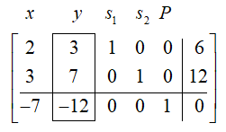
this order. Finally, the simplex method requires that the objective function be listed as the bottom line in the matrix so that we have:
\[
\begin{array}{c}\begin{array}{cccccc}
x\; & y\; & s_{1}\; & s_{2}\; & P\; & \; \end{array} \\
\left[\begin{array}{ccccc|c}
2 & 3 & 1 & 0 & 0 & 6 \\
3 & 7 & 0 & 1 & 0 & 12 \\
\hline-7 & -12 & 0 & 0 & 1 & 0
\end{array}\right] \end{array}
\nonumber\]

We have established the initial simplex tableau. Note that he horizontal and vertical lines are used simply to separate constraint coefficients from constants and objective function coefficients. Also notice that the slack variable columns, along with the objective function output, form the identity matrix.

Solving the Linear Programming Problem by Using the Initial Tableau

We will present the algorithm for solving, however, note that it is not entirely intuitive.

1. Select a pivot column
We first select a pivot column, which will be the column that contains the largest negative coefficient in the row containing the objective function. Note that the largest negative number belongs to the term that contributes most to the objective function. This is intentional since we want to focus on values that make the output as large as possible.
Our pivot is thus the \(y\) column.

2. Select a pivot row.
Do this by computing the ratio of each constraint constant to its respective coefficient in the pivot column - this is called the test ratio. Select the row with the smallest test ratio.

We first calculate the test ratios:

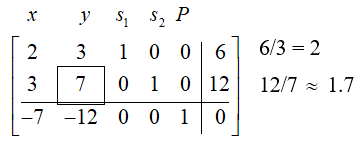
Since the test ratio is smaller for row 2, we select it as the pivot row. The boxed value is now called our pivot. To justify why we do this, observe that 2 and 1.7 are simply the vertical intercepts of the two inequalities. We select the smaller one to ensure we have a corner point that is in our feasible region.

3. Using Gaussian elimination

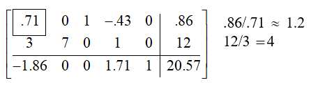
We next eliminate rows 1 and \(3 .\) We want to take \(-3 / 7\) multiplied by row 2 and add it to row 1 , so that we eliminate the 3 in the second column. We also want next to eliminate the \(-12\) in row \(3 .\) To do this, we must multiply 7 by \(12 / 7\)  and add it to row 3 (recall that placing the value you wish to cancel out in the denominator of a multiple and the value you wish to achieve in the numerator of the multiple, you obtain the new value).

We can see that we have effectively zeroed out the second column non-pivot values. We get the following matrix
\[
\left[\begin{array}{ccccc|c}
.71 & 0 & 1 & -.43 & 0 & .86 \\
3 & 7 & 0 & 1 & 0 & 12 \\
\hline-1.86 & 0 & 0 & 1.71 & 1 & 20.57
\end{array}\right]
\nonumber \]

What have we done? For one, we have maxed out the contribution of the \(2-2\) entry \(y-\) value coefficient to the objective function. Have we optimized the function? Not quite, as we still see that there is a negative value in the first column. This tells us that \(x\) can still contribute to the objective function. To eliminate this, we first find the pivot row by obtaining test ratios:

We proceed to eliminate all non-pivot values by multiplying the top row by \(-3 / 0.71\) and adding it to the second row, and adding \(1.86 / 0.71\) times the first row to the third row.

There remain no additional negative entries in the objective function row. We thus have the following matrix:
\[
\left[\begin{array}{ccccc|c}
.71 & 0 & 1 & -.43 & 0 & .86 \\
0 & 7 & -4.23 & 2.81 & 0 & 8.38 \\
\hline 0 & 0 & 2.62 & .59 & 1 & 22.82
\end{array}\right]
\nonumber\]
We are thus prepared to read the solutions.

4. To identify the solution set, focus we focus only on the columns with exactly one nonzero entry \(-\) these are called active variables (columns with more than one non-zero entry are thus called inactive variables)

We notice that both the \(x\) and \(y\) columns are active variables. We really don't care about the slack variables, much like we ignore inequalities when we are finding intersections. We now see that,

\[ \begin{align*} .71x + s_1 - .43{s_2} & = .86 \\ 7y - 4.23{s_1} + 2.81{s_2} & = 8.38\\  2.62{s_1} + .59{s_2} + P &= 22.82 \end{align*}\]

Setting the slack variables to 0, gives:

\[\begin{align*} .71x &= .86 &\to x \approx 1.21 \\ 7y &= 8.38 &\to y \approx 1.20\\ P &= 22.82& \end{align*}\]

Thus, the triplet, \(\left( x,y,z \right)\sim \left( 1.21,1.20,22.82 \right)\) is the solution to the linear programming problem. That is, inputs of 1.21 and 1.20 will yield a maximum objective function value of 22.82.

The entire process of solving using simplex method is:

Simplex Method

1. Set up the problem. That is, write the objective function and the constraints.
2. Convert the inequalities into equations. This is done by adding one slack variable for each inequality.
3. Construct the initial simplex tableau. Write the objective function as the bottom row.
4. The most negative entry in the bottom row identifies a column.
5. Calculate the quotients. The smallest quotient identifies a row. The element in the intersection of the column identified in step 4 and the row identified in this step is identified as the pivot element. The quotients are computed by dividing the far right column by the identified column in step 4. A quotient that is a zero, or a negative number, or that has a zero in the denominator, is ignored.
6. Perform pivoting to make all other entries in this column zero. This is done the same way as we did with the Gauss-Jordan method for matrices.
7. When there are no more negative entries in the bottom row, we are finished; otherwise, we start again from step 4.
8. Read off your answers. Get the variables using the columns with 1 and 0s. All other variables are zero. The maximum value you are looking for appears in the bottom right hand corner.

Exercise \(\PageIndex{1}\)

1.  Use simplex method to solve:

Maximize: \[P = 5x + 7y + 9z\nonumber \]

Subject to:

 \[\begin{align*} x + 4y + 2z &\leq 8  \\ 3x + 5y + z &\leq 6  \\ x \geq 0,y \geq 0,z &\geq 0  \\ \end{align*} \nonumber \]

Answer

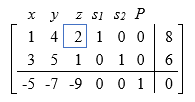
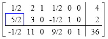
We set up the initial tableau.  The most negative entry in the bottom row is in the third column, so we select that column.  Calculating the quotients we have 8/2 = 4 in the first row, and 6/1 = 6 in the second row.  The smaller value is in row one, so we choose that row.  Our pivot is in row 1 column 3.

Now we perform the pivot.  We might start by scaling the top row by ½ to get a 1 in the pivot position.  Then we can add -1 times the top row to the second row, and 9 times the top row to the third row.

Now we are prepared to pivot again.  The most negative entry in the bottom row is in column 1, so we select that column.  Looking at the ratios, \(\frac{4}{1/2}=8\) and \(\frac{2}{5/2} =0.8\).  Choosing the smaller, we have our pivot in row 2 column 1.

We can multiply the second row by \(\frac{2}{5}\) to get a 1 in the pivot position, then add \(-\frac{1}{2}\) times the second row to the first row and \(\frac{1}{2}\) times the second row to the third row to reduce.

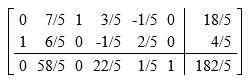
Only the first and third columns contain only one non-zero value and are active variables.  We set the remaining variables equal to zero and find our solution:

\[x = \frac{4}{5},\quad y = 0,\quad z = \frac{18}{5}\nonumber \]

Important Topics of this Section

Initial tableau

Pivot row and column

Simplex method

Reading the answer from a reduced tableau