
1.2: Echelon Forms
- Page ID
- 186282
\( \newcommand{\vecs}[1]{\overset { \scriptstyle \rightharpoonup} {\mathbf{#1}} } \)
\( \newcommand{\vecd}[1]{\overset{-\!-\!\rightharpoonup}{\vphantom{a}\smash {#1}}} \)
\( \newcommand{\dsum}{\displaystyle\sum\limits} \)
\( \newcommand{\dint}{\displaystyle\int\limits} \)
\( \newcommand{\dlim}{\displaystyle\lim\limits} \)
\( \newcommand{\id}{\mathrm{id}}\) \( \newcommand{\Span}{\mathrm{span}}\)
( \newcommand{\kernel}{\mathrm{null}\,}\) \( \newcommand{\range}{\mathrm{range}\,}\)
\( \newcommand{\RealPart}{\mathrm{Re}}\) \( \newcommand{\ImaginaryPart}{\mathrm{Im}}\)
\( \newcommand{\Argument}{\mathrm{Arg}}\) \( \newcommand{\norm}[1]{\| #1 \|}\)
\( \newcommand{\inner}[2]{\langle #1, #2 \rangle}\)
\( \newcommand{\Span}{\mathrm{span}}\)
\( \newcommand{\id}{\mathrm{id}}\)
\( \newcommand{\Span}{\mathrm{span}}\)
\( \newcommand{\kernel}{\mathrm{null}\,}\)
\( \newcommand{\range}{\mathrm{range}\,}\)
\( \newcommand{\RealPart}{\mathrm{Re}}\)
\( \newcommand{\ImaginaryPart}{\mathrm{Im}}\)
\( \newcommand{\Argument}{\mathrm{Arg}}\)
\( \newcommand{\norm}[1]{\| #1 \|}\)
\( \newcommand{\inner}[2]{\langle #1, #2 \rangle}\)
\( \newcommand{\Span}{\mathrm{span}}\) \( \newcommand{\AA}{\unicode[.8,0]{x212B}}\)
\( \newcommand{\vectorA}[1]{\vec{#1}} % arrow\)
\( \newcommand{\vectorAt}[1]{\vec{\text{#1}}} % arrow\)
\( \newcommand{\vectorB}[1]{\overset { \scriptstyle \rightharpoonup} {\mathbf{#1}} } \)
\( \newcommand{\vectorC}[1]{\textbf{#1}} \)
\( \newcommand{\vectorD}[1]{\overrightarrow{#1}} \)
\( \newcommand{\vectorDt}[1]{\overrightarrow{\text{#1}}} \)
\( \newcommand{\vectE}[1]{\overset{-\!-\!\rightharpoonup}{\vphantom{a}\smash{\mathbf {#1}}}} \)
\( \newcommand{\vecs}[1]{\overset { \scriptstyle \rightharpoonup} {\mathbf{#1}} } \)
\(\newcommand{\longvect}{\overrightarrow}\)
\( \newcommand{\vecd}[1]{\overset{-\!-\!\rightharpoonup}{\vphantom{a}\smash {#1}}} \)
\(\newcommand{\avec}{\mathbf a}\) \(\newcommand{\bvec}{\mathbf b}\) \(\newcommand{\cvec}{\mathbf c}\) \(\newcommand{\dvec}{\mathbf d}\) \(\newcommand{\dtil}{\widetilde{\mathbf d}}\) \(\newcommand{\evec}{\mathbf e}\) \(\newcommand{\fvec}{\mathbf f}\) \(\newcommand{\nvec}{\mathbf n}\) \(\newcommand{\pvec}{\mathbf p}\) \(\newcommand{\qvec}{\mathbf q}\) \(\newcommand{\svec}{\mathbf s}\) \(\newcommand{\tvec}{\mathbf t}\) \(\newcommand{\uvec}{\mathbf u}\) \(\newcommand{\vvec}{\mathbf v}\) \(\newcommand{\wvec}{\mathbf w}\) \(\newcommand{\xvec}{\mathbf x}\) \(\newcommand{\yvec}{\mathbf y}\) \(\newcommand{\zvec}{\mathbf z}\) \(\newcommand{\rvec}{\mathbf r}\) \(\newcommand{\mvec}{\mathbf m}\) \(\newcommand{\zerovec}{\mathbf 0}\) \(\newcommand{\onevec}{\mathbf 1}\) \(\newcommand{\real}{\mathbb R}\) \(\newcommand{\twovec}[2]{\left[\begin{array}{r}#1 \\ #2 \end{array}\right]}\) \(\newcommand{\ctwovec}[2]{\left[\begin{array}{c}#1 \\ #2 \end{array}\right]}\) \(\newcommand{\threevec}[3]{\left[\begin{array}{r}#1 \\ #2 \\ #3 \end{array}\right]}\) \(\newcommand{\cthreevec}[3]{\left[\begin{array}{c}#1 \\ #2 \\ #3 \end{array}\right]}\) \(\newcommand{\fourvec}[4]{\left[\begin{array}{r}#1 \\ #2 \\ #3 \\ #4 \end{array}\right]}\) \(\newcommand{\cfourvec}[4]{\left[\begin{array}{c}#1 \\ #2 \\ #3 \\ #4 \end{array}\right]}\) \(\newcommand{\fivevec}[5]{\left[\begin{array}{r}#1 \\ #2 \\ #3 \\ #4 \\ #5 \\ \end{array}\right]}\) \(\newcommand{\cfivevec}[5]{\left[\begin{array}{c}#1 \\ #2 \\ #3 \\ #4 \\ #5 \\ \end{array}\right]}\) \(\newcommand{\mattwo}[4]{\left[\begin{array}{rr}#1 \amp #2 \\ #3 \amp #4 \\ \end{array}\right]}\) \(\newcommand{\laspan}[1]{\text{Span}\{#1\}}\) \(\newcommand{\bcal}{\cal B}\) \(\newcommand{\ccal}{\cal C}\) \(\newcommand{\scal}{\cal S}\) \(\newcommand{\wcal}{\cal W}\) \(\newcommand{\ecal}{\cal E}\) \(\newcommand{\coords}[2]{\left\{#1\right\}_{#2}}\) \(\newcommand{\gray}[1]{\color{gray}{#1}}\) \(\newcommand{\lgray}[1]{\color{lightgray}{#1}}\) \(\newcommand{\rank}{\operatorname{rank}}\) \(\newcommand{\row}{\text{Row}}\) \(\newcommand{\col}{\text{Col}}\) \(\renewcommand{\row}{\text{Row}}\) \(\newcommand{\nul}{\text{Nul}}\) \(\newcommand{\var}{\text{Var}}\) \(\newcommand{\corr}{\text{corr}}\) \(\newcommand{\len}[1]{\left|#1\right|}\) \(\newcommand{\bbar}{\overline{\bvec}}\) \(\newcommand{\bhat}{\widehat{\bvec}}\) \(\newcommand{\bperp}{\bvec^\perp}\) \(\newcommand{\xhat}{\widehat{\xvec}}\) \(\newcommand{\vhat}{\widehat{\vvec}}\) \(\newcommand{\uhat}{\widehat{\uvec}}\) \(\newcommand{\what}{\widehat{\wvec}}\) \(\newcommand{\Sighat}{\widehat{\Sigma}}\) \(\newcommand{\lt}{<}\) \(\newcommand{\gt}{>}\) \(\newcommand{\amp}{&}\) \(\definecolor{fillinmathshade}{gray}{0.9}\)We saw how to translate a system of linear equations into an augmented matrix; now we want to find an algorithm for “solving” such an augmented matrix. First. we must decide what it means for an augmented matrix to be “solved”.
A matrix is in row-echelon form if:
- All zero rows are at the bottom.
- The first nonzero entry of a row is to the right of the first nonzero entry of the row above.
- Below the first nonzero entry of a row, all entries are zero.
Here is a picture of a matrix in row-echelon form:
\[\left[\begin{array}{ccccc} \color{red}{\boxed{\star}} &\star &\star &\star &\star \\ 0&\color{red}{\boxed{\star}} & \star &\star &\star \\ 0&0&0&\color{red}{\boxed{\star}} &\star \\ 0&0&0&0&0 \end{array}\right] \qquad \begin{aligned} \star &= \text{any number} \\ \color{red}\boxed\star &= \text{any nonzero number} \end{aligned} \nonumber \]
A pivot is the first nonzero entry of a row of a matrix in row-echelon form.
A matrix in row-echelon form is generally easy to solve using back-substitution. For example,
\[\left[\begin{array}{ccc|c} 1 &2& 3& 6\\ 0& 1& 2& 4 \\ 0& 0& 10& 30 \end{array}\right]\quad\xrightarrow{\text{becomes}}\quad \left\{\begin{array}{rrrrrrr} x &+& 2y &+& 3z &=& 6 \\ {}&{}& y &+& 2z& =& 4 \\ {}&{}&{}&{}& 10z &=& 30. \end{array}\right. \nonumber\]
We immediately see that \(z=3\text{,}\) which implies \(y = 4-2\cdot 3 = -2\) and \(x = 6 - 2(-2) - 3\cdot 3 = 1.\) See Example \(\PageIndex{3}\).
A matrix is in reduced row-echelon form if it is in row-echelon form, and in addition:
- Each pivot is equal to 1.
- Each pivot is the only nonzero entry in its column.
Here is a picture of a matrix in reduced row-echelon form:
\[\left[\begin{array}{ccccc} \color{red}{1} &0&\star &0&\star \\ 0&\color{red}{1} &\star &0 &\star \\ 0&0&0&\color{red}{1}&\star \\ 0&0&0&0&0\end{array}\right] \qquad \begin{aligned} \star &= \text{any number} \\ \color{red}1 &= \text{pivot} \end{aligned} \nonumber\]
A matrix in reduced row-echelon form is in some sense completely solved. For example,
\[\left[\begin{array}{ccc|c} 1 &0& 0& 1\\ 0& 1& 0& -2\\ 0& 0& 1& 3\end{array}\right] \quad\xrightarrow{\text{becomes}}\quad \left\{\begin{array}{rrr} x &=& 1\\ y &=& -2 \\ z &=& 3.\end{array}\right. \nonumber \]
The following matrices are in reduced row-echelon form:
\[\left[\begin{array}{ccc}1&0&2 \\ 0&1&-1\end{array}\right]\qquad \left[\begin{array}{cccc}0&1&8&0\end{array}\right] \qquad \left[\begin{array}{cc|c} 1&17&0\\0&0&1\end{array}\right]\qquad\left[\begin{array}{ccc}0&0&0\\0&0&0\end{array}\right]\nonumber\]
The following matrices are in row-echelon form but not reduced row-echelon form:
\[\left[\begin{array}{cc}2&1\\0&1\end{array}\right]\qquad \left[\begin{array}{ccc|c} 2&7&1&4 \\ 0&0&2&1 \\ 0&0&0&3\end{array}\right]\qquad \left[\begin{array}{ccc}1&17&0\\0&1&1\end{array}\right] \qquad \left[\begin{array}{ccc}2&1&3\\0&0&0\end{array}\right]\nonumber\]
The following matrices are not in echelon form:
\[\left[\begin{array}{ccc|c} 2&7&1&4\\0&0&2&1\\0&0&1&3 \end{array}\right]\qquad\left[\begin{array}{cc|c}0&17&0\\0&2&1\end{array}\right]\qquad\left[\begin{array}{cc}2&1\\2&1\end{array}\right] \qquad \left[\begin{array}{c}0\\1\\0\\0\end{array}\right]\nonumber\]
When deciding if an augmented matrix is in (reduced) row-echelon form, there is nothing special about the augmented column(s). Just ignore the vertical line.
If an augmented matrix is in reduced row-echelon form, the corresponding linear system is viewed as solved. We will see below why this is the case, and we will show that any matrix can be put into reduced row-echelon form using only row operations.
Every matrix is row-equivalent to one and only one matrix in reduced row-echelon form.
We will give an algorithm, called row reduction or Gaussian elimination, which demonstrates that every matrix is row-equivalent to at least one matrix in reduced row-echelon form.
The uniqueness statement is interesting—it means that, no matter how you row reduce, you always get the same matrix in reduced row-echelon form.
This assumes, of course, that you only do the three legal row operations, and you don’t make any arithmetic errors.
We will not prove uniqueness, but maybe you can!
- Step 1a: Swap the 1st row with a lower one so a leftmost nonzero entry is in the 1st row (if necessary).
- Step 1b: Scale the 1st row so that its first nonzero entry is equal to 1.
- Step 1c: Use row replacement so all entries below this 1 are 0.
- Step 2a: Swap the 2nd row with a lower one so that the leftmost nonzero entry is in the 2nd row.
- Step 2b: Scale the 2nd row so that its first nonzero entry is equal to 1.
- Step 2c: Use row replacement so all entries below this 1 are 0.
- Step 3a: Swap the 3rd row with a lower one so that the leftmost nonzero entry is in the 3rd row.
- etc.
- Last Step: Use row replacement to clear all entries above the pivots, starting with the last pivot.
Row reduce this matrix:
\[\left[\begin{array}{ccc|c} 0&-7&-4&2 \\ 2&4&6&12\\ 3&1&-1&-2\end{array}\right]\nonumber\]
Solution
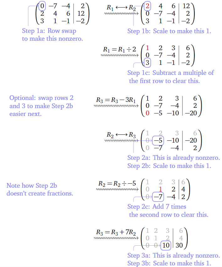
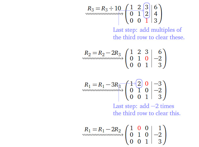
The reduced row-echelon form of the matrix is
\[\boxed{\left[\begin{array}{ccc|c}1&0&0&1 \\ 0&1&0&-2\\0&0&1&3\end{array}\right] }\quad\xrightarrow{\text{translates to}}\quad \left\{\begin{array}{rrrrrrr} x&{}&{}&{}&{}&=&1 \\ {}&{}&y&{}&{}&=&-2 \\ {}&{}&{}&{}&z&=&3\end{array}\right.\nonumber\]
The reduced row-echelon form of the matrix tells us that the only solution is \((x,y,z)= (1,-2,3)\)
Here is the row-reduction algorithm, summarized in pictures.
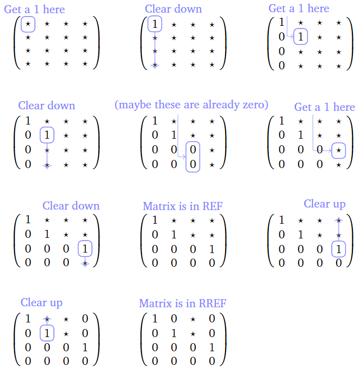
Figure \(\PageIndex{3}\)
It will be very important to know where the pivots of a matrix after row reducing are; this is the reason for the following piece of terminology.
A pivot position of a matrix is an entry that is a pivot of a row-echelon form of that matrix.
A pivot column of a matrix is a column that contains a pivot position.
Find the pivot positions and pivot columns of this matrix
\[A=\left[\begin{array}{ccc|c} 0 &-7& -4& 2\\ 2& 4& 6& 12 \\ 3& 1& -1& -2\end{array}\right]\nonumber\]
Solution
We saw in Example \(\PageIndex{5}\) that a row-echelon form of the matrix is
\[\left[\begin{array}{ccc|c} 1 &2& 3& 6\\ 0& 1& 2& 4\\ 0& 0& 10& 30\end{array}\right]\nonumber\]
The pivot positions of \(A\) are the entries that become pivots in a row-echelon form; they are marked in red below:
\[\left[\begin{array}{ccc|c}\color{red}{0}&-7&-4&2 \\ 2&\color{red}{4}&6&12 \\ 3&1&\color{red}{-1}&-2\end{array}\right]\nonumber\]
The first, second, and third columns are pivot columns.
If we attempt to solve the linear system
\[\left\{\begin{array}{rrrrr}2x &+& 10y &=& -1 \\ 3x &+& 15y &=& 2\end{array}\right. \nonumber \]
using row reduction, we see:
\[\begin{align*} \left[\begin{array}{cc|c} 2&10&-1 \\ 3&15&2 \end{array}\right] \quad\xrightarrow{R_1=R_1\div 2}\quad & \left[\begin{array}{cc|c} \color{red}{1}&5&{-\frac{1}{2}} \\ 3&15&2 \end{array}\right] &&\color{blue}{\text{(Step 1b)}} \\ {} \quad\xrightarrow{R_2=R_2-3R_1}\quad & \left[\begin{array}{cc|c} 1&5&{-\frac{1}{2}} \\ \color{red}{0} &0&{\frac{7}{2}} \end{array}\right] &&\color{blue}{\text{(Step 1c)}} \\ {}\quad\xrightarrow{R_2=R_2\times\frac 27}\quad & \left[\begin{array}{cc|c} 1&5&{-\frac{1}{2}} \\ 0&0&\color{red}{1} \end{array}\right] &&\color{blue}{\text{(Step 2b)}} \\ {} \quad\xrightarrow{R_1=R_1+\frac 12R_2}\quad & \left[\begin{array}{cc|c} 1&5&\color{red}{0} \\ 0&0&1\end{array}\right] &&\color{blue}{\text{(Step 2c)}}\end{align*}\]
This row-reduced matrix corresponds to the inconsistent system
\[\left\{\begin{array}{rrrrr} x &+& 5y &=& 0\\ & &0& =& 1 \end{array}\right. \nonumber \]
In the above example, we saw how to recognize the reduced row-echelon form of an inconsistent system.
An augmented matrix corresponds to an inconsistent system of equations if and only if the last column (i.e., the augmented column) is a pivot column.
In other words, the row-reduced matrix of an inconsistent system looks like this:
\[\left[\begin{array}{cccc|c} 1&0&\star &\star &\color{red}{0} \\ 0&1&\star &\star &\color{red}{0}\\ 0&0&0&0&\color{red}{1}\end{array}\right]\nonumber\]
We have discussed two classes of matrices so far:
- When the reduced row-echelon form of a matrix has a pivot in every non-augmented column, then it corresponds to a system with a unique solution:
\[\left[\begin{array}{ccc|c} 1 &0& 0& 1\\ 0& 1& 0& -2\\ 0& 0& 1& 3\end{array}\right] \quad\xrightarrow{\text{translates to}}\quad \left\{\begin{array}{rrrrrrc} x&{}&{}&{}&{}&=&1 \\ {}&{}&y&{}&{}&=&-2 \\ {}&{}&{}&{}&z&=&3\end{array}\right. \nonumber\] - When the reduced row-echelon form of a matrix has a pivot in the last (augmented) column, then it corresponds to a system with no solutions:
\[\left[\begin{array}{cc|c} 1&5&0 \\ 0&0&1\end{array}\right] \quad\xrightarrow{\text{translates to}}\quad \left\{\begin{array}{rrrrrrl} x &+& 5y &=& 0 \\ {}&{}& 0 &=& 1\end{array}\right.\nonumber\]