2.3: Partial Derivatives

When studying derivatives of functions of one variable, we found that one interpretation of the derivative is an instantaneous rate of change of \(y\) as a function of \(x.\) Leibniz notation for the derivative is \(\dfrac{dy}{dx},\) which implies that \(y\) is the dependent variable and \(x\) is the independent variable. For a function \(z=f(x,y)\) of two variables, \(x\) and \(y\) are the independent variables and \(z\) is the dependent variable. This raises two questions right away: How do we adapt Leibniz notation for functions of two variables? Also, what is an interpretation of the derivative? The answer lies in partial derivatives.

Definition: Partial Derivatives

Let \(f(x,y)\) be a function of two variables. Then the partial derivative of \(f\) with respect to \(x\), written as \(∂f/∂x\) or \(f_x,\) is defined as

\[\dfrac{∂f}{∂x}=f_x(x,y)=\lim_{h→0}\dfrac{f(x+h,y)−f(x,y)}{h} \nonumber \]

The partial derivative of \(f\) with respect to \(y\), written as \(\dfrac{\partial f}{\partial y}\) or \(f_y,\) is defined as

\[\dfrac{∂f}{∂y}=f_y(x,y)=\lim_{k→0}\dfrac{f(x,y+k)−f(x,y)}{k} \nonumber\]

This definition shows two differences already. First, the notation changes, in the sense that we still use a version of Leibniz notation, but the \(d\) in the original notation is replaced with the symbol \(∂\). (This rounded \(“d”\) is usually called “partial,” so \(\dfrac{∂f}{∂x}\) is spoken as the “partial of \(f\) with respect to \(x\).”) This is the first hint that we are dealing with partial derivatives. Second, we now have two different derivatives we can take, since there are two different independent variables. Depending on which variable we choose, we can come up with different partial derivatives altogether, and often do.

Example \(\PageIndex{1}\): Calculating Partial Derivatives from the Definition

Use the definition of the partial derivative as a limit to calculate \(\dfrac{∂f}{∂x}\) and \(\dfrac{∂f}{∂y}\) for the function

\[f(x,y)=x^2−3xy+2y^2−4x+5y−12 \nonumber \]

Solution

First, calculate \(f(x+h,y)\):

\[\begin{align*} f(x+h,y) &=(x+h)^2−3(x+h)y+2y^2−4(x+h)+5y−12 \\ &=x^2+2xh+h^2−3xy−3hy+2y^2−4x−4h+5y−12 \end{align*} \nonumber \]

Next, substitute this into the formula for \(\dfrac{∂f}{∂x}\) and simplify:

\[\begin{align*} \dfrac{∂f}{∂x} &=\lim_{h→0}\dfrac{f(x+h,y)−f(x,y)}{h} \\
&=\lim_{h→0}\dfrac{(x^2+2hx+h^2−3xy−3hy+2y^2−4x−4h+5y−12)−(x^2−3xy+2y^2−4x+5y−12)}{h} \\ &=\lim_{h→0}\dfrac{x^2+2hx+h^2−3xy−3hy+2y^2−4x−4h+5y−12−x^2+3xy−2y^2+4x−5y+12}{h} \\
&=\lim_{h→0}\dfrac{2hx+h^2−3hy−4h}{h}\\
&=\lim_{h→0}\dfrac{h(2x+h−3y−4)}{h} \\
&=\lim_{h→0}(2x+h−3y−4) \\
&=2x−3y−4 \end{align*}\]

To calculate \(\dfrac{∂f}{∂y}\), first calculate \(f(x,y+k)\):

\[\begin{align*} f(x,y+k) &=x^2−3x(y+k)+2(y+k)^2−4x+5(y+k)−12 \\ &=x^2−3xy−3xk+2y^2+4yk+2k^2−4x+5y+5k−12 \end{align*}\]

Next, substitute this into the formula for \(\dfrac{∂f}{∂y}\) and simplify:

\[ \begin{align*} \dfrac{∂f}{∂y} &=\lim_{k→0}\dfrac{f(x,y+k)−f(x,y)}{k} \\
&=\lim_{k→0}\dfrac{(x^2−3xy−3xk+2y^2+4yk+2k^2−4x+5y+5k−12)−(x^2−3xy+2y^2−4x+5y−12)}{k} \\ &=\lim_{k→0}\dfrac{x^2−3xy−3xk+2y^2+4yk+2k^2−4x+5y+5k−12−x^2+3xy−2y^2+4x−5y+12}{k} \\
&=\lim_{k→0}\dfrac{−3xk+4yk+2k^2+5k}{k} \\
&=\lim_{k→0}\dfrac{k(−3x+4y+2k+5)}{k} \\
&=\lim_{k→0}(−3x+4y+2k+5) \\
&=−3x+4y+5 \end{align*}\]

The idea to keep in mind when calculating partial derivatives is to treat all independent variables, other than the variable with respect to which we are differentiating, as constants. Then proceed to differentiate as with a function of a single variable. To see why this is true, first fix \(y\) and define \(g(x)=f(x,y)\) as a function of \(x\). Then

\[g′(x) =\lim_{h→0}\dfrac{g(x+h)−g(x)}{h}=\lim_{h→0}\dfrac{f(x+h,y)−f(x,y)}{h} =\dfrac{∂f}{∂x} \nonumber \]

The same is true for calculating the partial derivative of \(f\) with respect to \(y\). This time, fix \(x\) and define \(h(y)=f(x,y)\) as a function of \(y\). Then

\[h′(x) =\lim_{k→0}\dfrac{h(x+k)−h(x)}{k}=\lim_{k→0}\dfrac{f(x,y+k)−f(x,y)}{k} =\dfrac{∂f}{∂y} \nonumber \]

This means that all of the previously learned differentiation rules and shortcuts still apply!

Example \(\PageIndex{2}\): Calculating Partial Derivatives

Calculate \(\dfrac{∂f}{∂x}\) and \(\dfrac{∂f}{∂y}\) for the following functions by holding the opposite variable constant then differentiating:

(a) \(f(x,y)=x^2−3xy+2y^2−4x+5y−12\)

(b) \(f(x,y)=\sin(x^2y−2x+4)\)

(c) \(f(x,y)=x^2e^{xy}\)

Solution:

a. To calculate \(\dfrac{∂f}{∂x}\), treat the variable \(y\) as a constant. Then differentiate \(f(x,y)\) with respect to \(x\) using the sum, difference, and power rules:

\[\dfrac{∂f}{∂x} =\dfrac{∂}{∂x}\left[x^2−3xy+2y^2−4x+5y−12\right] =2x−3y+0−4+0−0 =2x−3y−4 \nonumber \]

The derivatives of the third, fifth, and sixth terms are all zero because they do not contain the variable \(x\), so they are treated as constant terms. The derivative of the second term is equal to the coefficient of \(x\), which is \(−3y\).

Calculating \(\dfrac{∂f}{∂y}\):

\[\dfrac{∂f}{∂y} =\dfrac{∂}{∂y}\left[x^2−3xy+2y^2−4x+5y−12\right] =0−3x+4y−0+5−0 =−3x+4y+5 \nonumber \]

These are the same answers obtained in Example \(\PageIndex{1}\).

(b) To calculate \(\dfrac{∂f}{∂x}\), treat the variable \(y\) as a constant. Then differentiate \(f(x,y)\) with respect to \(x\) using the chain rule and power rule:

\[\dfrac{∂f}{∂x} =\dfrac{∂}{∂x}\left[\sin(x^2y−2x+4)\right]=\cos(x^2y−2x+4)\cdot \left(\dfrac{∂}{∂x}[x^2y−2x+4]\right)=(2xy−2)\cos(x^2y−2x+4) \nonumber \]

To calculate \(\dfrac{∂f}{∂y}\), treat the variable \(x\) as a constant. Then differentiate \(f(x,y)\) with respect to \(y\) using the chain rule and power rule:

\[ \dfrac{∂f}{∂y} =\dfrac{∂}{∂y}\left[\sin(x^2y−2x+4)\right]=\cos(x^2y−2x+4)\cdot \dfrac{∂}{∂y}[x^2y−2x+4] =x^2\cos(x^2y−2x+4) \nonumber \]

(c) To calculate \(\dfrac{∂f}{∂x}\), treat the variable \(y\) as a constant. Then differentiate \(f(x,y)\) with respect to \(x\) using the product rule and chain rule:

\[\dfrac{∂f}{∂x} =\dfrac{∂}{∂x}\left[x^2e^{xy}\right]= \dfrac{∂}{∂x}[x^2]\cdot e^{xy}+x^2\cdot \dfrac{∂}{∂x}[e^{xy}] = 2xe^{xy}+x^2\left( e^{xy}\cdot \dfrac{∂}{∂x}[xy]\right)=2xe^{xy}+x^2\cdot e^{xy}\cdot y=(2x+x^2y)e^{xy} \nonumber \]

To calculate \(\dfrac{∂f}{∂y}\), treat the variable \(x\) as a constant. Then differentiate \(f(x,y)\) with respect to \(y\) using the product rule and chain rule:

\[\dfrac{∂f}{∂y} =\dfrac{∂}{∂y}\left[x^2e^{xy}\right]= \dfrac{∂}{∂y}[x^2]\cdot e^{xy}+x^2\cdot \dfrac{∂}{∂y}[e^{xy}] = 0\cdot e^{xy}+x^2\left( e^{xy}\cdot \dfrac{∂}{∂y}[xy]\right)=0+x^2\cdot e^{xy}\cdot x=x^3e^{xy} \nonumber \]

How can we interpret these partial derivatives? Recall that the graph of a function of two variables is a surface in \(\mathbb{R}^3\). If we remove the limit from the definition of the partial derivative with respect to \(x\), the difference quotient remains:

\[\dfrac{f(x+h,y)−f(x,y)}{h}. \nonumber \]

This resembles the difference quotient for the derivative of a function of one variable, except for the presence of the \(y\) variable. Figure \(\PageIndex{1}\) illustrates a surface described by an arbitrary function \(z=f(x,y).\)

Figure \(\PageIndex{1}\): Secant line passing through the points \((x,y,f(x,y))\) and \((x+h,y,f(x+h,y)).\)

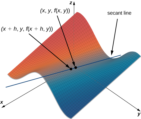
In the figure above, the value of \(h\) is positive. If we graph \(f(x,y)\) and \(f(x+h,y)\) for an arbitrary point \((x,y),\) then the slope of the secant line passing through these two points is given by

\[\dfrac{f(x+h,y)−f(x,y)}{h} \nonumber \]

This line is parallel to the \(x\)-axis. Therefore, the slope of the secant line represents an average rate of change of the function \(f\) as we travel parallel to the \(x\)-axis. As \(h\) approaches zero, the slope of the secant line approaches the slope of the tangent line.

If we choose to change \(y\) instead of \(x\) by the same incremental value \(h\), then the secant line is parallel to the \(y\)-axis and so is the tangent line. Therefore, \(\dfrac{\partial f}{\partial x}\) represents the slope of the tangent line passing through the point \((x,y,f(x,y))\) parallel to the \(x\)-axis and \(\dfrac{\partial f}{\partial y}\) represents the slope of the tangent line passing through the point \((x,y,f(x,y))\) parallel to the \(y\)-axis. (Later, if we wish to find the slope of a tangent line passing through the same point in any other direction, we will define the concept of a directional derivative.)

Suppose we have a function of three variables, such as \(w=f(x,y,z).\) We can calculate partial derivatives of \(w\) with respect to any of the independent variables, simply as extensions of the definitions for partial derivatives of functions of two variables.

Definition: Partial Derivatives

Let \(f(x,y,z)\) be a function of three variables. Then, the partial derivative of \(f\) with respect to \(x\), written as \(\dfrac{∂f}{∂x},\) or \(f_x,\) is defined to be

\[\dfrac{∂f}{∂x}=f_x(x,y,z)=\lim_{h→0}\dfrac{f(x+h,y,z)−f(x,y,z)}{h} \nonumber \]

The partial derivative of \(f\) with respect to \(y\), written as \(\dfrac{∂f}{∂y}\), or \(f_y\), is defined to be

\[\dfrac{∂f}{∂y}=f_y(x,y,z)=\lim_{k→0}\dfrac{f(x,y+k,z)−f(x,y,z)}{k} \nonumber \]

The partial derivative of \(f\) with respect to \(z\), written as \(\dfrac{∂f}{∂z}\), or \(f_z\), is defined to be

\[\dfrac{∂f}{∂z}=f_z(x,y,z)=\lim_{m→0}\dfrac{f(x,y,z+m)−f(x,y,z)}{m} \nonumber \]

We can calculate a partial derivative of a function of three variables using the same idea we used for a function of two variables. For example, if we have a function \(f\) of \(x,y\), and \(z\), and we wish to calculate \(\dfrac{∂f}{∂x}\), then we treat the other two independent variables as if they are constants, then differentiate with respect to \(x\).

Example \(\PageIndex{3}\): Calculating Partial Derivatives for a Function of Three Variables

Calculate the three partial derivatives of the following functions.

(a) \(f(x,y,z)=\dfrac{x^2y−4xz+y^2}{x−3yz}\)

(b) \(g(x,y,z)=\sin(x^2y−z)+\cos(x^2−yz)\)

Solution

(a) Treat all variables as constants except the one whose partial derivative you are calculating:

\[\begin{align*} \dfrac{∂f}{∂x} &=\dfrac{∂}{∂x}\left[\dfrac{x^2y−4xz+y^2}{x−3yz}\right] \\[6pt]
&=\dfrac{\dfrac{∂}{∂x}(x^2y−4xz+y^2)(x−3yz)−(x^2y−4xz+y^2)\dfrac{∂}{∂x}(x−3yz)}{(x−3yz)^2} \\[6pt]
&=\dfrac{(2xy−4z)(x−3yz)−(x^2y−4xz+y^2)(1)}{(x−3yz)^2} \\[6pt]
&=\dfrac{x^2y−6xy^2z+12yz^2−y^2}{(x−3yz)^2} \end{align*}\]

\[\begin{align*} \dfrac{∂f}{∂y} &=\dfrac{∂}{∂y}\left[\dfrac{x^2y−4xz+y^2}{x−3yz}\right] \\[6pt]
&=\dfrac{\dfrac{∂}{∂y}(x^2y−4xz+y^2)(x−3yz)−(x^2y−4xz+y^2)\dfrac{∂}{∂y}(x−3yz)}{(x−3yz)^2} \\[6pt]
&=\dfrac{(x^2+2y)(x−3yz)−(x^2y−4xz+y^2)(−3z)}{(x−3yz)^2} \\[6pt]
&=\dfrac{x^3+2xy−3y^2z−12xz^2}{(x−3yz)^2} \end{align*}\]

\[\begin{align*} \dfrac{∂f}{∂z} &=\dfrac{∂}{∂z}\left[\dfrac{x^2y−4xz+y^2}{x−3yz}\right] \\[6pt]
&=\dfrac{\dfrac{∂}{∂z}(x^2y−4xz+y^2)(x−3yz)−(x^2y−4xz+y^2)\dfrac{∂}{∂z}(x−3yz)}{(x−3yz)^2} \\[6pt]
&=\dfrac{(−4x)(x−3yz)−(x^2y−4xz+y^2)(−3y)}{(x−3yz)^2} \\[6pt]
&=\dfrac{−4x^2+3x^2y^2+3y^3}{(x−3yz)^2} \end{align*}\]

(b) Treat all variables as constants except the one whose partial derivative you are calculating:

\[\begin{align*} \dfrac{∂f}{∂x} &=\dfrac{∂}{∂x} \left[\sin(x^2y−z)+\cos(x^2−yz) \right] \\[6pt]
&=(\cos(x^2y−z))\dfrac{∂}{∂x}(x^2y−z)−(\sin(x^2−yz))\dfrac{∂}{∂x}(x^2−yz) \\[6pt]
&=2xy\cos(x^2y−z)−2x\sin(x^2−yz) \end{align*}\]

\[\begin{align*} \dfrac{∂f}{∂y} &=\dfrac{∂}{∂y}[\sin(x^2y−z)+\cos(x^2−yz)] \\[6pt]
&=(\cos(x^2y−z))\dfrac{∂}{∂y}(x^2y−z)−(\sin(x^2−yz))\dfrac{∂}{∂y}(x^2−yz) \\[6pt]
&=x^2\cos(x^2y−z)+z\sin(x^2−yz) \end{align*}\]

\[\begin{align*} \dfrac{∂f}{∂z} &=\dfrac{∂}{∂z}[\sin(x^2y−z)+\cos(x^2−yz)] \\[6pt]
&=(\cos(x^2y−z))\dfrac{∂}{∂z}(x^2y−z)−(\sin(x^2−yz))\dfrac{∂}{∂z}(x^2−yz) \\[6pt]
&=−\cos(x^2y−z)+y\sin(x^2−yz) \end{align*} \nonumber \]

Consider the function

\[f(x,y)=2x^3−4xy^2+5y^3−6xy+5x−4y+12 \nonumber \]

Its partial derivatives are

\[\dfrac{∂f}{∂x}=6x^2−4y^2−6y+5 \text{ and } \dfrac{∂f}{∂y}=−8xy+15y^2−6x−4 \nonumber \]

Each of these partial derivatives is a function of two variables, so we can calculate partial derivatives of these functions. Just as with derivatives of single-variable functions, we can call these second-order derivatives, third-order derivatives, and so on. In general, they are referred to as higher-order partial derivatives. There are four second-order partial derivatives for any function (provided they all exist):

\[\dfrac{∂^2f}{∂x^2} =\dfrac{∂}{∂x}\left[\dfrac{∂f}{∂x}\right]=f_{xx} \hspace{.3in}
\dfrac{∂^2f}{∂y∂x} =\dfrac{∂}{∂y}\left[\dfrac{∂f}{∂x}\right]=f_{xy} \hspace{.3in}
\dfrac{∂^2f}{∂x∂y} =\dfrac{∂}{∂x}\left[\dfrac{∂f}{∂y}\right]=f_{yx} \hspace{.3in}
\dfrac{∂^2f}{∂y^2} =\dfrac{∂}{∂y}\left[\dfrac{∂f}{∂y}\right]=f_{yy} \nonumber \]

Higher-order partial derivatives calculated with respect to different variables, such as \(f_{xy}\) and \(f_{yx}\), are commonly called mixed partial derivatives.

Example \(\PageIndex{4}\): Calculating Second Partial Derivatives

Calculate all four second partial derivatives for the function \(f(x,y)=xe^{−3y}+\sin(2x−5y) \)

Solution:

To calculate \(f_{xx}\) and \(f_{xy}\), we first calculate \(f_x\):

\[\dfrac{∂f}{∂x}=e^{−3y}+2\cos(2x−5y) \nonumber \]

To calculate \(f_{xx}\), differentiate \(f_x\) above with respect to \(x\):

\[f_{xx}=\dfrac{∂}{∂x}\left[f_x\right] =\dfrac{∂}{∂x}[e^{−3y}+2\cos(2x−5y)]=−4\sin(2x−5y) \nonumber \]

To calculate \(f_{xy}\), differentiate \(f_x\) with respect to \(y\):

\[f_{xy}=\dfrac{∂}{∂y}\left[f_x\right] =\dfrac{∂}{∂y}[e^{−3y}+2\cos(2x−5y)] =−3e^{−3y}+10\sin(2x−5y) \nonumber \]

To calculate \(f_{yx}\) and \(f_{yy}\), first calculate \(f_y\):

\[\dfrac{∂f}{∂y}=−3xe^{−3y}−5\cos(2x−5y) \nonumber \]

To calculate \(f_{yx} \), differentiate \(f_y\) above with respect to \(x\):

\[f_{yx}=\dfrac{∂}{∂x} \left[f_y\right] =\dfrac{∂}{∂x}[−3xe^{−3y}−5\cos(2x−5y)]=−3e^{−3y}+10\sin(2x−5y) \nonumber \]

To calculate \(f_{yy} \), differentiate \(f_y\) with respect to \(y\):

\[f_{yy}=\dfrac{∂}{∂y}\left[f_y\right] =\dfrac{∂}{∂y}[−3xe^{−3y}−5\cos(2x−5y)] =9xe^{−3y}−25\sin(2x−5y) \nonumber \]

At this point we should notice that, in the Example above, it was true that \(\dfrac{∂^2f}{∂y∂x}=\dfrac{∂^2f}{∂x∂y}\). Under certain conditions, this is always true. In fact, it is a direct consequence of the following theorem.

Theorem \(\PageIndex{1}\): Equality of Mixed Partial Derivatives (Clairaut’s Theorem)

Suppose that \(f(x,y)\) is defined on an open disk \(D\) that contains the point \((a,b)\). If the functions \(f_{xy}\) and \(f_{yx}\) are continuous on \(D\), then \(f_{xy}(a,b)=f_{yx}(a,b)\).

Clairaut’s theorem guarantees that as long as mixed second-order derivatives are continuous, the order in which we choose to differentiate the functions (i.e., which variable goes first, then second, and so on) does not matter. It can be extended to higher-order derivatives as well. The proof of Clairaut’s theorem can be found in most Advanced Calculus books.

Two other second-order partial derivatives can be calculated for any function \(f(x,y).\) The partial derivative \(f_{xx}\) is equal to the partial derivative of \(f_x\) with respect to \(x\), and \(f_{yy}\) is equal to the partial derivative of \(f_y\) with respect to \(y\).