
4.4: The Divergence Theorem
- Page ID
- 191860

\( \newcommand{\vecs}[1]{\overset { \scriptstyle \rightharpoonup} {\mathbf{#1}} } \)
\( \newcommand{\vecd}[1]{\overset{-\!-\!\rightharpoonup}{\vphantom{a}\smash {#1}}} \)
\( \newcommand{\dsum}{\displaystyle\sum\limits} \)
\( \newcommand{\dint}{\displaystyle\int\limits} \)
\( \newcommand{\dlim}{\displaystyle\lim\limits} \)
\( \newcommand{\id}{\mathrm{id}}\) \( \newcommand{\Span}{\mathrm{span}}\)
( \newcommand{\kernel}{\mathrm{null}\,}\) \( \newcommand{\range}{\mathrm{range}\,}\)
\( \newcommand{\RealPart}{\mathrm{Re}}\) \( \newcommand{\ImaginaryPart}{\mathrm{Im}}\)
\( \newcommand{\Argument}{\mathrm{Arg}}\) \( \newcommand{\norm}[1]{\| #1 \|}\)
\( \newcommand{\inner}[2]{\langle #1, #2 \rangle}\)
\( \newcommand{\Span}{\mathrm{span}}\)
\( \newcommand{\id}{\mathrm{id}}\)
\( \newcommand{\Span}{\mathrm{span}}\)
\( \newcommand{\kernel}{\mathrm{null}\,}\)
\( \newcommand{\range}{\mathrm{range}\,}\)
\( \newcommand{\RealPart}{\mathrm{Re}}\)
\( \newcommand{\ImaginaryPart}{\mathrm{Im}}\)
\( \newcommand{\Argument}{\mathrm{Arg}}\)
\( \newcommand{\norm}[1]{\| #1 \|}\)
\( \newcommand{\inner}[2]{\langle #1, #2 \rangle}\)
\( \newcommand{\Span}{\mathrm{span}}\) \( \newcommand{\AA}{\unicode[.8,0]{x212B}}\)
\( \newcommand{\vectorA}[1]{\vec{#1}} % arrow\)
\( \newcommand{\vectorAt}[1]{\vec{\text{#1}}} % arrow\)
\( \newcommand{\vectorB}[1]{\overset { \scriptstyle \rightharpoonup} {\mathbf{#1}} } \)
\( \newcommand{\vectorC}[1]{\textbf{#1}} \)
\( \newcommand{\vectorD}[1]{\overrightarrow{#1}} \)
\( \newcommand{\vectorDt}[1]{\overrightarrow{\text{#1}}} \)
\( \newcommand{\vectE}[1]{\overset{-\!-\!\rightharpoonup}{\vphantom{a}\smash{\mathbf {#1}}}} \)
\( \newcommand{\vecs}[1]{\overset { \scriptstyle \rightharpoonup} {\mathbf{#1}} } \)
\(\newcommand{\longvect}{\overrightarrow}\)
\( \newcommand{\vecd}[1]{\overset{-\!-\!\rightharpoonup}{\vphantom{a}\smash {#1}}} \)
\(\newcommand{\avec}{\mathbf a}\) \(\newcommand{\bvec}{\mathbf b}\) \(\newcommand{\cvec}{\mathbf c}\) \(\newcommand{\dvec}{\mathbf d}\) \(\newcommand{\dtil}{\widetilde{\mathbf d}}\) \(\newcommand{\evec}{\mathbf e}\) \(\newcommand{\fvec}{\mathbf f}\) \(\newcommand{\nvec}{\mathbf n}\) \(\newcommand{\pvec}{\mathbf p}\) \(\newcommand{\qvec}{\mathbf q}\) \(\newcommand{\svec}{\mathbf s}\) \(\newcommand{\tvec}{\mathbf t}\) \(\newcommand{\uvec}{\mathbf u}\) \(\newcommand{\vvec}{\mathbf v}\) \(\newcommand{\wvec}{\mathbf w}\) \(\newcommand{\xvec}{\mathbf x}\) \(\newcommand{\yvec}{\mathbf y}\) \(\newcommand{\zvec}{\mathbf z}\) \(\newcommand{\rvec}{\mathbf r}\) \(\newcommand{\mvec}{\mathbf m}\) \(\newcommand{\zerovec}{\mathbf 0}\) \(\newcommand{\onevec}{\mathbf 1}\) \(\newcommand{\real}{\mathbb R}\) \(\newcommand{\twovec}[2]{\left[\begin{array}{r}#1 \\ #2 \end{array}\right]}\) \(\newcommand{\ctwovec}[2]{\left[\begin{array}{c}#1 \\ #2 \end{array}\right]}\) \(\newcommand{\threevec}[3]{\left[\begin{array}{r}#1 \\ #2 \\ #3 \end{array}\right]}\) \(\newcommand{\cthreevec}[3]{\left[\begin{array}{c}#1 \\ #2 \\ #3 \end{array}\right]}\) \(\newcommand{\fourvec}[4]{\left[\begin{array}{r}#1 \\ #2 \\ #3 \\ #4 \end{array}\right]}\) \(\newcommand{\cfourvec}[4]{\left[\begin{array}{c}#1 \\ #2 \\ #3 \\ #4 \end{array}\right]}\) \(\newcommand{\fivevec}[5]{\left[\begin{array}{r}#1 \\ #2 \\ #3 \\ #4 \\ #5 \\ \end{array}\right]}\) \(\newcommand{\cfivevec}[5]{\left[\begin{array}{c}#1 \\ #2 \\ #3 \\ #4 \\ #5 \\ \end{array}\right]}\) \(\newcommand{\mattwo}[4]{\left[\begin{array}{rr}#1 \amp #2 \\ #3 \amp #4 \\ \end{array}\right]}\) \(\newcommand{\laspan}[1]{\text{Span}\{#1\}}\) \(\newcommand{\bcal}{\cal B}\) \(\newcommand{\ccal}{\cal C}\) \(\newcommand{\scal}{\cal S}\) \(\newcommand{\wcal}{\cal W}\) \(\newcommand{\ecal}{\cal E}\) \(\newcommand{\coords}[2]{\left\{#1\right\}_{#2}}\) \(\newcommand{\gray}[1]{\color{gray}{#1}}\) \(\newcommand{\lgray}[1]{\color{lightgray}{#1}}\) \(\newcommand{\rank}{\operatorname{rank}}\) \(\newcommand{\row}{\text{Row}}\) \(\newcommand{\col}{\text{Col}}\) \(\renewcommand{\row}{\text{Row}}\) \(\newcommand{\nul}{\text{Nul}}\) \(\newcommand{\var}{\text{Var}}\) \(\newcommand{\corr}{\text{corr}}\) \(\newcommand{\len}[1]{\left|#1\right|}\) \(\newcommand{\bbar}{\overline{\bvec}}\) \(\newcommand{\bhat}{\widehat{\bvec}}\) \(\newcommand{\bperp}{\bvec^\perp}\) \(\newcommand{\xhat}{\widehat{\xvec}}\) \(\newcommand{\vhat}{\widehat{\vvec}}\) \(\newcommand{\uhat}{\widehat{\uvec}}\) \(\newcommand{\what}{\widehat{\wvec}}\) \(\newcommand{\Sighat}{\widehat{\Sigma}}\) \(\newcommand{\lt}{<}\) \(\newcommand{\gt}{>}\) \(\newcommand{\amp}{&}\) \(\definecolor{fillinmathshade}{gray}{0.9}\)Before examining the divergence theorem, it is helpful to begin with an overview of the versions of the Fundamental Theorem of Calculus we have discussed:
- The Fundamental Theorem of Calculus: \[\int_a^b f' (x) \, dx = f(b) - f(a) \nonumber \] This theorem relates the integral of derivative \(f'\) over line segment \([a,b]\) along the \(x\)-axis to a difference in \(f\) evaluated at the boundary points.
- The Fundamental Theorem for Line Integrals: \[\int_C \nabla f \cdot d\vecs r = f(P_1) - f(P_0) \nonumber \] where \(P_0\) is the initial point of \(C\) and \(P_1\) is the terminal point of \(C\). The Fundamental Theorem for Line Integrals allows a curve \(C\) to be any path in a plane or in space, not just a line segment on the \(x\)-axis. If we think of the gradient as a derivative, then this theorem relates an integral of derivative \( \nabla f\) over path \(C\) to a difference of \(f\) evaluated on the boundary of \(C\).
- Green’s theorem: \[\iint_D (Q_x - P_y)\,dA = \int_C \vecs F \cdot d\vecs r \nonumber \] Since \(Q_x - P_y = \text{curl } (\vecs F) \cdot \mathbf{\hat k}\) and curl is a derivative-like operator, Green’s theorem relates the integral of the derivative \(\text{curl}(\vecs F)\) over planar region \(D\) to an integral of \(\vecs F\) over the boundary of \(D\).
- Stokes’ theorem: \[\iint_S \text{curl}(\vecs F ) \cdot d\vecs S = \int_C \vecs F \cdot d\vecs r \nonumber \] If we think of the curl as a derivative of sorts, then Stokes’ theorem relates the integral of derivative \(\text{curl}(\vecs F )\) over surface \(S\) (not necessarily planar) to an integral of \(\vecs F\) over the boundary of \(S\).
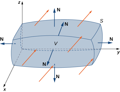
The divergence theorem follows the general pattern of these other theorems. If we think of divergence as a derivative of sorts, then the divergence theorem relates a triple integral of derivative \(\text{div}(\vecs F )\) over a solid to a flux integral of \(\vecs F\) over the boundary of the solid. More specifically, the divergence theorem relates a flux integral of vector field \(\vecs F\) over a closed surface \(S\) to a triple integral of the divergence of \(\vecs F\) over the solid enclosed by \(S\).
Let \(S\) be a piecewise, smooth closed surface that encloses solid \(E\) in space. Assume that \(S\) is oriented outward, and let \(\vecs F\) be a vector field with continuous partial derivatives on an open region containing \(E\). Then
\[\iiint_E \text{div}(\vecs F )\, dV = \iint_S \vecs F \cdot d\vecs S \nonumber \]
The proof of the divergence theorem is beyond the scope of this text. However, we look at an informal proof that gives a general feel for why the theorem is true, but does not prove the theorem with full rigor. This explanation follows the informal explanation given for why Stokes’ theorem is true.
Let \(B\) be a small box with sides parallel to the coordinate planes inside \(E\). Let the center of \(B\) have coordinates \((x,y,z)\) and suppose the edge lengths are \(\Delta x, \, \Delta y\), and \(\Delta z\). The normal vector out of the top of the box is \(\mathbf{\hat k}\) and the normal vector out of the bottom of the box is \(-\mathbf{\hat k}\). The dot product of \(\vecs F = \langle P, Q, R \rangle\) with \(\mathbf{\hat k}\) is \(R\) and the dot product with \(-\mathbf{\hat k}\) is \(-R\). The area of the top of the box (and the bottom of the box) \(\Delta S\) is \(\Delta x \Delta y\).
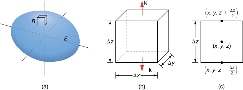
The flux out of the top of the box can be approximated by \(R \left(x,\, y,\, z + \dfrac{\Delta z}{2}\right) \,\Delta x \,\Delta y\) and the flux out of the bottom of the box is \(- R \left(x,\, y,\, z - \dfrac{\Delta z}{2}\right) \,\Delta x \,\Delta y\). If we denote the difference between these values as \(\Delta R\), then the net flux in the vertical direction can be approximated by \(\Delta R\, \Delta x \,\Delta y\). However,
\[\Delta R \,\Delta x \,\Delta y = \left(\dfrac{\Delta R}{\Delta z}\right) \,\Delta x \,\Delta y \Delta z \approx \left(\dfrac{\partial R}{\partial z}\right) \,\Delta V \nonumber \]
Therefore, the net flux in the vertical direction can be approximated by \(\left(\dfrac{\partial R}{\partial z}\right)\Delta V\). Similarly, the net flux in the \(x\)-direction can be approximated by \(\left(\dfrac{\partial P}{\partial x}\right)\,\Delta V\) and the net flux in the \(y\)-direction can be approximated by \(\left(\dfrac{\partial Q}{\partial y}\right)\,\Delta V\). Adding the fluxes in all three directions gives an approximation of the total flux out of the box:
\[\text{Total flux }\approx \left(\dfrac{\partial P}{\partial x} + \dfrac{\partial Q}{\partial y} + \dfrac{\partial R}{\partial z} \right) \Delta V = \text{div}(\vecs F ) \,\Delta V \nonumber \]
This approximation becomes arbitrarily close to the value of the total flux as the volume of the box shrinks to zero.
The sum of \(\text{div}(\vecs F )\,\Delta V\) over all the small boxes approximating \(E\) is approximately \(\displaystyle \iiint_E \text{div}(\vecs F )\,dV\). On the other hand, the sum of \(\text{div}(\vecs F )\,\Delta V\) over all the small boxes approximating \(E\) is the sum of the fluxes over all these boxes. Just as in the informal proof of Stokes’ theorem, adding these fluxes over all the boxes results in the cancellation of a lot of the terms. If an approximating box shares a face with another approximating box, then the flux over one face is the negative of the flux over the shared face of the adjacent box. These two integrals cancel out. When adding up all the fluxes, the only flux integrals that survive are the integrals over the faces approximating the boundary of \(E\). As the volumes of the approximating boxes shrink to zero, this approximation becomes arbitrarily close to the flux over \(S\).
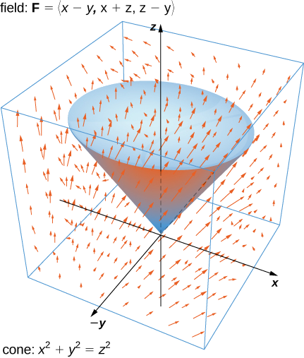
Verify the divergence theorem for vector field \(\vecs F = \langle x - y, \, x + z, \, z - y \rangle\) and surface \(S\) that consists of cone \(x^2 + y^2 = z^2, \, 0 \leq z \leq 1\), and the circular top of the cone (see the following figure). Assume this surface is positively oriented.
Solution
Let \(E\) be the solid cone enclosed by \(S\). To verify the theorem for this example, we show that
\[\iiint_E \text{div} (\vecs F ) \,dV = \iint_S \vecs F \cdot d\vecs S\nonumber \]
by calculating each integral separately.
To compute the triple integral, note that \(\text{div}( \vecs F )= P_x + Q_y + R_z = 2\), and therefore the triple integral is
\[ \iiint_E \text{div} (\vecs F ) \, dV = \iiint_E 2 dV = 2 \cdot \text{Volume} (E) =2\cdot \dfrac{\pi}{3}(1)^2(1)=\dfrac{2\pi}{3} \nonumber \]
(Recall the volume of a right circular cone is given by \(\dfrac{\pi}{3} r^2 h\) and this cone has \(h = r = 1\).)
To compute the flux integral, first note that \(S\) is piecewise smooth; \(S\) can be written as a union of smooth surfaces. Therefore, we break the flux integral into two pieces: one flux integral across the circular top of the cone and one flux integral across the remaining portion of the cone. Call the circular top \(S_1\) and the portion under the top \(S_2\). We start by calculating the flux across the circular top of the cone. Notice that \(S_1\) has parameterization
\[\vecs r(u,v) = \langle u \cos(v), u\sin(v),1 \rangle \quad \text{ for } \quad \, 0 \leq u \leq 1, \, 0 \leq v \leq 2\pi \nonumber \]
Then, the tangent vectors are \(\vecs r_u = \langle \cos (v), \sin (v), 0 \rangle \) and \(\vecs r_v = \langle -u \sin(v), u\cos(v), 0 \rangle \). Thus \(\vecs{r}_u\times \vecs{r}_v = \langle 0,0,u\rangle \).
This has upward orientation, which is outward for our full surface \(S\) and therefore is positively oriented. Now we find the flux across \(S_1\) is:
\[ \begin{align*} \iint_{S_1} \vecs F \cdot d\vecs S &= \int_0^1 \int_0^{2\pi} \vecs F (\vecs r ( u,v)) \cdot (\vecs r_u \times \vecs r_v) \, dA \\[4pt] &= \int_0^1 \int_0^{2\pi} \langle u \cos(v)-u\sin(v), u\cos(v)+1, 1-u\sin(v) \rangle \cdot \langle 0,0,u \rangle \, dv\, du \\[4pt] &= \int_0^1 \int_0^{2\pi} \left( u - u^2 \sin (v) \right)\, dv \, du \\[4pt] &= \int_0^1 \left[ uv + u^2 \cos (v) \right. \Big|_0^{2\pi} \, du \\[4pt] &= \int_0^1 2\pi u \, du \\[4pt] &= \left[ \pi u^2 \right.\Big|_0^1 \\[4pt] &= \pi \end{align*}\]
We now calculate the flux over \(S_2\). A parameterization of this surface is
\[\vecs r(u,v) = \langle u\cos(v), u\sin(v), u \rangle \quad \text{ for } \quad 0 \leq u \leq 1, \, 0 \leq v \leq 2\pi \nonumber \]
The tangent vectors are \(\vecs r_u = \langle \cos (v), \, \sin (v), \, 1 \rangle \) and \(\vecs r_v = \langle -u\sin(v), u\cos(v),0 \rangle \), so \(\vecs{r}_u\times \vecs{r}_v = \langle - u \cos(v),-u\sin(v), u \rangle \).
This points upward, which is inward for our full surface \(S\) and therefore is negatively oriented. We multiply it by \(-1\) to make it outward, and now we find the flux across \(S_2\) is:
\[ \begin{align*} \iint_{S_2} \vecs F \cdot d\vecs S &= \int_0^1 \int_0^{2\pi} \vecs F ( \vecs r ( u,v)) \cdot \left(-(\vecs r_u \times \vecs r_v)\right) \, dA \\[4pt] &= \int_0^1 \int_0^{2\pi} \langle u\cos(v)-u\sin(v), u\cos(v)+u, u-u\sin(v) \rangle \cdot \langle u\cos(v), u\sin(v), -u \rangle\,dv\,du \\[4pt] &= \int_0^1 \int_0^{2\pi} \left( u^2 \cos^2 (v) + 2u^2 \sin (v) - u^2\right) \,dv\,du \\[4pt] &= \int_0^1 \int_0^{2\pi} \left(\dfrac{1}{2}u^2 \cos (2v) + 2u^2 \sin (v) - \dfrac{1}{2}u^2\right) \,dv\,du \\[4pt] &= \int_0^1 \left[ \dfrac{1}{4}u^2 \sin (2v) - 2u^2 \cos (v) - \dfrac{1}{2}u^2v \right|_0^{2\pi} \,du \\[4pt] &= \int_0^1 - \pi u^2 \,du \\[4pt] &= \left[ -\dfrac{\pi}{3} u^3\right|_0^1 \\[4pt] &= -\frac{\pi}{3} \end{align*}\]
We have found total flux across \(S\) is
\[\iint_{S} \vecs F \cdot d\vecs S = \iint_{S_1}\vecs F \cdot d\vecs S + \iint_{S_2} \vecs F \cdot d\vecs S = \pi +\left(-\dfrac{\pi}{3}\right)= \frac{2\pi}{3} = \iiint_E \text{div}\left( \vecs F\right) \,dV\nonumber \]
and we have verified the divergence theorem for this example.
Verify the divergence theorem for vector field \(\vecs F = \langle 2y^2 , 3x^2, 5z^3 \rangle\) and surface \(S\) that consists of the unit sphere.
Solution
Let \(E\) be the solid unit sphere enclosed by \(S\). To verify the theorem for this example, we show that
\[\iiint_E \text{div} (\vecs F ) \,dV = \iint_S \vecs F \cdot d\vecs S\nonumber \]
by calculating each integral separately.
To compute the triple integral, note that \(\text{div}( \vecs F )= P_x + Q_y + R_z = 15z^2 \), and therefore the triple integral is
\[\begin{align*} \iiint_E \text{div} (\vecs F ) \, dV &= \iiint_E 15z^2 dV \\[4pt] &= \int_0^1 \int_0^\pi \int_0^{2\pi} 15(\rho \cos(\phi ))^2 \, \rho^2 \sin(\phi )\, d\theta \, d\phi \, d\rho \\[4pt] &= \int_0^1 \int_0^\pi \int_0^{2\pi} 15 \rho^4 \cos^2 (\phi ) \sin(\phi )\, d\theta \, d\phi \, d\rho \\[4pt] &=\left( \int_0^1 15 \rho^4 d\rho \right) \left( \int_0^\pi \cos^2 (\phi ) \sin(\phi )\, d\phi \right) \left( \int_0^{2\pi} \, d\theta \right) \\[4pt] &= \left[ 3 \rho^5 \right. \Big|_0^1 \cdot \left[ -\dfrac{1}{3}\cos^3(\phi) \right|_0^\pi \cdot \left[ \theta \right. \Big|_0^{2\pi} \\[4pt] &= 3 \cdot \left( \dfrac{2}{3} \right) \cdot 2\pi \\[4pt] &= 4\pi \end{align*}\]
To compute the flux integral, first note that \(S\) is smooth and can be parameterized using spherical coordinates (with \(\rho =1\) ) as:
\[\vecs r(u,v) = \langle \sin(u)\cos(v), \sin(u)\sin(v), \cos(u) \rangle \quad \text{ for } \quad \, 0 \leq u \leq \pi, \, 0 \leq v \leq 2\pi \nonumber \]
We find \(\vecs r_u = \langle \cos(u)\cos(v), \cos(u)\sin(v), -\sin(u) \rangle \) and \(\vecs r_v = \langle -\sin(u) \sin(v), \sin(u)\cos(v), 0 \rangle \).
Next we calculate \(\vecs{r}_u\times \vecs{r}_v = \langle \sin^2(u)\cos(v), \sin^2(u)\sin(v), \sin(u)\cos(u) \rangle \).
This has outward orientation for our surface \(S\) and therefore is positively oriented. Now we find the flux across \(S\) is:
\[ \begin{align*} \iint_{S} \vecs F \cdot d\vecs S &= \int_0^{\pi} \int_0^{2\pi} \vecs F (\vecs r ( u,v)) \cdot (\vecs r_u \times \vecs r_v) \, dA \\[4pt]
&= \int_0^{\pi} \int_0^{2\pi} \langle 2\sin^2(u)\sin^2(v), 3\sin^2(u)\cos^2(v), 5\cos^3(u) \rangle \cdot \langle \sin^2(u)\cos(v), \sin^2(u)\sin(v), \sin(u)\cos(u) \rangle \, dv\, du \\[4pt]
&= \int_0^{\pi} \int_0^{2\pi} \left(2\sin^4(u)\sin^2(v)\cos(v)+2\sin^4(u)\cos^2(v)\sin(v)+5\cos^4(u)\sin(u)\right) \, dv \, du \\[4pt] &= \int_0^{\pi} \left[ \dfrac{2}{3}\sin^4(u)\sin^3(v) -\dfrac{2}{3}\sin^4(u)\cos^3(v) +5v\cos^4(u)\sin(u) \right. \Big|_0^{2\pi} \, du \\[4pt] &= \int_0^{\pi} 10\pi \cos^4(u)\sin(u) \, du \\[4pt] &= \left[ -2\pi \cos^5(u) \right. \Big|_0^{\pi}\\[4pt] &= 4 \pi \end{align*}\]
Once more, we have verified the divergence theorem holds in this example.
Let \(\vecs F = \left\langle - \dfrac{y}{z}, \, \dfrac{x}{z}, \, 0 \right\rangle\) and \(E=\left\{ (x,y,z)\, \mid \,1 \leq x \leq 4, \, 2 \leq y \leq 5, \, 1 \leq z \leq 4\right\} \). If \(S\) is the boundary of this cube oriented outward, find the flux of \(\vecs{F}\) on \(S\).
Solution
The flux across the boundary of this cube requires six separate parameterizations and calculations.
Instead, we use the Divergence Theorem:
\[\iint_S \vecs F \cdot d\vecs S = \iiint_E \text{div}(\vecs F ) \, dV = \iiint_E 0 \, dV = 0 \nonumber \]
Therefore the flux is zero.
The example above illustrates a remarkable consequence of the divergence theorem. Let \(S\) be a piecewise, smooth closed surface and let \(\vecs F\) be a vector field defined on an open region containing the surface enclosed by \(S\). If \(\vecs F\) has the form \(F = \langle f (y,z), \, g(x,z), \, h(x,y)\rangle\), then the divergence of \(\vecs F\) is zero. By the divergence theorem, the flux of \(\vecs F\) across \(S\) is also zero. This makes certain flux integrals incredibly easy to calculate. For example, suppose we wanted to calculate the flux integral \(\displaystyle \iint_S \vecs F \cdot d\vecs S\) where \(S\) is any closed surface and
\[\vecs F = \langle \sin (y) \, e^{yz}, \, x^2z^2, \, \cos (xy) \, e^{\sin (x)} \rangle \nonumber \]
Calculating the flux integral directly would be difficult, if not impossible, using techniques we studied previously. At the very least, we would have to parameterize a surface (or many surfaces, if we are unlucky). But, because the divergence of this field is zero, the divergence theorem immediately shows that the flux integral is zero.
Another way to consider this is in terms of Stokes' Theorem. Any vector field \(\vecs{F}\) with a divergence of zero can be written as the curl of some \(\vecs{G}\). If \(S\) is a closed surface, then its "boundary" can be considered to be empty (or a single point), which means the line integral along this boundary should be zero.
Find the volume of the region contained inside of the torus with major radius \(M\) and minor radius \(m\) (where \(M>m\)).

Solution
The volume of any region \(E\) can be represented by a triple integral \(\displaystyle \iiint_E 1\, dV\).
Unfortunately, this region is incredibly difficult to describe in rectangular, cylindrical, and spherical coordinates. Instead, we look to parameterize the surface of \(E\) and use the Divergence Theorem!
We parameterize using \(\vecs{r}(u,v)=\langle (m\cos(v)+M)\cos(u), (m\cos(v)+M)\sin(u), m\sin(v) \rangle\) for \(0\le u \le 2\pi, \, 0\le v \le 2\pi\).
\[ \vecs{r}_u = \langle -(m\cos(v)+M)\sin(u), (m\cos(v)+M)\cos(u),0\rangle \quad \text{ and } \quad \vecs{r}_v = \langle -m\sin(v)\cos(u), -m\sin(v)\sin(u), m\cos(v) \rangle \nonumber \]
The cross product of these vectors is therefore:
\[ \vecs{r}_u \times \vecs{r}_v = \langle m(m\cos(v)+M)\cos(v)\cos(u), m(m\cos(v)+M)\cos(v)\sin(u), m(m\cos(v)+M)\sin(v)\rangle \nonumber \]
Plugging in \(u=0,v=0\) we see that at \(\vecs{r}(0,0)=(M+m,0,0)\) we have \(\vecs{r}_u\times \vecs{r}_v = \langle m(m+M),0,0\rangle\), so this surface is parameterized outward, as needed for the Divergence Theorem. Next we need to find a vector field \(\vecs{F}\) such that \(\text{div}(\vecs{F})=1\), and \(\displaystyle \iint_S \vecs{F}\cdot d\vecs{S}\) is reasonable.
Looking at the normal vector \(\vecs{r}_u\times\vecs{r}_v\), the easiest choice should be \(\vecs{F}=\langle 0,0,z\rangle\):
\[ \begin{align*} \iiint_E 1\, dV &= \iiint_E \text{div} (\vecs{F})\, dV \\[4pt]
&= \iint_S \vecs{F}\cdot d\vecs{S} \\[4pt]
&= \int_0^{2\pi} \int_0^{2\pi} \langle 0,0, m\sin(v)\rangle \cdot \langle m(m\cos(v)+M)\cos(v)\cos(u), m(m\cos(v)+M)\cos(v)\sin(u), m(m\cos(v)+M)\sin(v)\rangle \, dA \\[4pt]
&= \int_0^{2\pi} \int_0^{2\pi} m^2(m\cos(v)+M)\sin^2(v) \, du \, dv \\[4pt]
&= \left( \int_0^{2\pi} m^2 \, du \right) \left( \int_0^{2\pi} \left( m\sin^2(v)\cos(v) +M\left( \dfrac{1}{2}-\dfrac{1}{2}\cos(2v)\right)\right) \, dv \right) \\[4pt]
&= \left[ m^2u \right. \Big|_0^{2\pi} \cdot \left[ \dfrac{m}{3} \sin^3(v)+\dfrac{M}{2}\left( v-\dfrac{1}{2}\sin(2v)\right) \right|_0^{2\pi} \\[4pt]
&= 2\pi m^2\cdot M\pi \\[4pt] &= 2Mm^2\pi^2 \end{align*} \]
Thus the volume of a torus is \(2Mm^2\pi^2\). Notice this can be written as the product of the area of the smaller circles (\(\pi m^2\)) and the circumference of the larger circle \(2\pi M\). Intuitively, the torus is simply a circular cylinder of radius \(m\) and height \(2\pi M\) bent around so that its top and bottom are touching.
Let \(M>0\) be a constant, and \(g(t),f(t)\) be functions bounded by \(0\le g(t)\le M\) and \(f(t)\ge 0\), which satisfy \(g(0)=g(2\pi)\) and \(f(0)=f(2\pi)\). Find the volume of the region contained inside of the surface parameterized by
\[ \vecs{r}(u,v)=\langle (g(u)\cos(v)+M)\cos(u), (g(u)\cos(v)+M)\sin(u), f(u)\sin(v) \rangle \quad \text{ for } \quad 0\le u \le 2\pi, \, 0\le v \le 2\pi \nonumber \]
Solution
This region is similar to a torus, but the smaller circular cross sections are replaced by ellipses with varying height and width.
Again, this region is incredibly difficult to describe in rectangular, cylindrical, and spherical coordinates. We find the tangent vectors:
\[ \vecs{r}_u = \langle g'(u)\cos(v)\cos(u)-(g(u)\cos(v)+M)\sin(u), g'(u)\cos(v)\sin(u)+(g(u)\cos(v)+M)\cos(u),f'(u)\sin(v) \rangle \nonumber \]
\[\vecs{r}_v = \langle -g(u)\sin(v)\cos(u), -g(u)\sin(v)\sin(u), f(u)\cos(v) \rangle \nonumber \]
The cross product of these vectors is therefore:
\[\begin{align*} \vecs{r}_u \times \vecs{r}_v &= \left[g'(u)f(u)\cos^2(v)\sin(u)+g(u)f(u)\cos^2(v)\cos(u)+Mf(u)\cos(v)\cos(u)+g(u)f'(u)\sin^2(v)\sin(u) \right] \, \mathbf{\hat{i}} \\
& - \left[ g'(u)f(u)\cos^2(v)\cos(u)-g(u)f(u)\cos^2(v)\sin(u)-Mf(u)\cos(v)\sin(u)+g(u)f'(u)\sin^2(v)\cos(u) \right] \, \mathbf{\hat{j}} \\
&+ \left[ g(u)(g(u)\cos(v) +M )\sin(v)\right] \, \mathbf{\hat{k}} \end{align*} \]
Once again, this surface is parameterized outward, as needed for the Divergence Theorem.
Next, we need to find a vector field \(\vecs{F}\) such that \(\text{div}(\vecs{F})=1\), and \(\displaystyle \iint_S \vecs{F}\cdot d\vecs{S}\) is reasonable.
Looking at the normal vector \(\vecs{r}_u\times\vecs{r}_v\), the obvious choice should again be \(\vecs{F}=\langle 0,0,z\rangle\):
\[ \begin{align*} \text{Volume} &= \iint_S \vecs{F}\cdot d\vecs{S} \\[4pt]
&= \int_0^{2\pi} \int_0^{2\pi} \langle 0,0, f(u)\sin(v) \rangle \cdot (\vecs{r}_u\times \vecs{r}_v ) \, dA \\[4pt]
&= \int_0^{2\pi} \int_0^{2\pi} f(u)g(u)(g(u)\cos(v) +M )\sin^2(v) \, dv \, du \\[4pt]
&= \int_0^{2\pi} \int_0^{2\pi} \left( f(u)\left[g(u)\right]^2 \sin^2(v)\cos(v) +Mf(u)g(u)\left( \dfrac{1}{2}-\dfrac{1}{2}\cos(2v)\right) \right) \, dv \, du \\[4pt]
&= \int_0^{2\pi} \left[ \dfrac{1}{3} f(u)\left[g(u)\right]^2 \sin^3(v) +Mf(u)g(u)\left( \dfrac{1}{2}v-\dfrac{1}{4}\sin(2v)\right) \right]_0^{2\pi} \, du \\[4pt]
&= \int_0^{2\pi} M\pi f(u)g(u) \, du \end{align*} \]
Notice that in our previous example, the torus has \(h(t)=g(t)=m\), which matches the result we would get from this more general formula.
In the case where \(M=5\), \(f(t)=\cos(2t)+3\) and \(g(t)=\cos(2t)+2\), we get a shape like the one below:

And since \(\displaystyle \int_0^{2\pi} f(u)g(u)\, du = \int_0^{2\pi} \left( \cos^2(2u)+5\cos(2u)+6\right) \, du = 13\pi\), we know the volume of this solid is \(V=65\pi^2\).
If instead we use \(M=10\), \(f(t)=2(t-\pi)^2\) and \(g(t)=(t-\pi)^2\) the shape looks like:

And since \(\displaystyle \int_0^{2\pi} f(u)g(u)\, du = \int_0^{2\pi} 2(u-\pi)^4 \, du = \dfrac{4\pi^5}{5}\), we know the volume of this solid is \(V=8\pi^6\).
It is important to recognize that the Divergence Theorem only applies to closed surfaces. If a surface \(S\) is not closed, however, we can always close it by adding on additional surfaces.
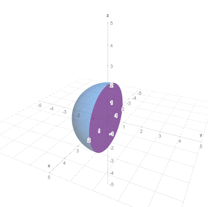
Find the flux of \(\vecs{F}=\langle e^{y^2}, 1, 3yz \rangle \) over the hemisphere \(S=\{ (x,y,z) \, \mid \, x^2+y^2+z^2=4, \, y\le 0\}\) oriented outward.
Solution
While we can parameterize \(S\) a few different ways, none of them yield a surface integral that is pleasant to solve directly.

Since \(S\) is not closed, we cannot immediately use the Divergence Theorem to avoid this flux integral. We remedy this by adding on a surface \(S_1\) to close the object. As long as it is oriented outwards, if we denote \(E\) as the region between them, we will have:
\[ \iiint_E \text{div}(\vecs{F})\, dV= \iint_S \vecs{F}\cdot d\vecs{S} + \iint_{S_1} \vecs{F}\cdot d\vecs{S} \nonumber \]
The simplest such surface is a flat disc on the \(y=0\) plane.
This surface is easy to parameterize, we can use \(\vecs{r}(u,v)=\langle u,0,v\rangle\) over \(D=\left\{ (u,v) \, \mid \, u^2+v^2\le 4\right\}\).
To find the flux over \(S_1\) we first find its tangent vectors: \(\vecs{r}_u=\mathbf{\hat{i}}\) and \(\vecs{r}_v=\mathbf{\hat{k}}\).
Therefore we have \(\vecs{r}_u\times \vecs{r}_v=-\mathbf{\hat{j}}\). Note that this points inward, so we will replace it with \(\mathbf{\hat{j}}\):
\[ \iint_{S_1} \vecs{F}\cdot d\vecs{r} = \iint_D \langle 1,1,0\rangle \cdot \mathbf{\hat{j}} \, dA= \iint_D 1\, dA= \text{area}(D)=4\pi \nonumber \]
The region between these surfaces is \(E=\left\{ (\rho \sin(\phi)\cos(\theta), \rho \sin(\phi)\sin(\theta), \rho \cos(\phi) )\, \mid \, 0\le \rho \le 2, \, 0\le \phi \le \pi, \, \pi \le \theta \le 2\pi \right\} \).
It is easy to calculate \(\text{div} (\vecs{F}))=3y\), so our triple integral becomes:
\[ \begin{align*} \iiint_E \text{div} (\vecs{F}) \, dV &= \iiint_E 3y\, dV \\[4pt]
&= \int_0^2 \int_0^\pi \int_\pi^{2\pi} 3\rho \sin(\phi)\sin(\theta )\, \rho^2 \sin(\phi) \, d\theta \, d\phi \, d\rho \\[4pt]
&= \left( \int_0^2 3\rho^3 \, d\rho \right) \left( \int_0^\pi \sin^2(\phi) \, d\phi \right) \left( \int_\pi^{2\pi} \sin(\theta) \, d\theta \right) \\[4pt]
&= \left[ \dfrac{3}{4}\rho^4 \right|_0^2 \cdot \left[ \dfrac{1}{2}\phi -\dfrac{1}{4}\sin(2\phi) \right|_0^\pi\cdot \left[ -\cos(\theta) \right. \Big|_\pi^{2\pi} \\[4pt]
&= 12\cdot \dfrac{\pi}{2} \cdot (-2)=-12\pi \end{align*} \]
Putting these all together, we see that
\[ \iint_S \vecs{F}\cdot d\vecs{r} = \iiint_E \text{div}(\vecs{F})\, dV - \iint_{S_1} \vecs{F}\cdot d\vecs{r} =-12\pi -4\pi =-16\pi \nonumber \]
The Divergence Theorem is a powerful tool that helps us to avoid many undesirable flux integral calculations. It acts as the capstone theorem of this text and demonstrates that the Fundamental Theorem of Calculus generalizes to many forms (as we summarized in the Overview of Theorems above). While integrals may come in many forms in multivariable calculus, we see that the "right kind" of derivative can cancel out with one layer of the "right kind" of integral in almost every one of them.
The divergence theorem relates the flux integral of closed surface \(S\) to a triple integral over the solid \(E\) which is enclosed by \(S\). Therefore, the theorem allows us to compute flux integrals or triple integrals that would ordinarily be difficult to compute by translating the flux integral into a triple integral and vice versa.
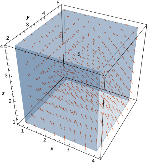
Example \(\PageIndex{3}\): Applying the Divergence Theorem
If \(S\) is cylinder \( x^2 + y^2 = 1, \, 0 \leq z \leq 2\), including the circular top and bottom, and \(\vecs F = \left\langle \dfrac{x^3}{3} + yz, \, \dfrac{y^3}{3} - \sin (xz), \, z - x - y \right\rangle\), find
\[\iint_S \vecs F \cdot d\vecs S \nonumber \]
Solution
We could calculate this integral without the divergence theorem, but the calculation is not straightforward because we would have to break the flux integral into three separate integrals: one for the top of the cylinder, one for the bottom, and one for the side. Furthermore, each integral would require parameterizing the corresponding surface, calculating tangent vectors and their cross product.
By contrast, the divergence theorem allows us to calculate the single triple integral over the solid enclosed by the cylinder, which we denote as \(E\).
In cylindrical coordinates, we have \(E=\left\{ (r\cos(\theta),r\sin(\theta),z)\, \mid \, 0\le r\le 1,\, 0\le \theta \le 2\pi, \, 0\le z\le 2 \right\}\). Therefore
\[ \begin{align*} \iint_S \vecs F \cdot d\vecs S &= \iiint_E \text{div}(\vecs F) \, dV \\[4pt]
&= \iiint_E (x^2 + y^2 + 1) \, dV \\[4pt]
&= \int_0^{2\pi} \int_0^1 \int_0^2 (r^2 + 1) \, r \, dz \, dr \, d\theta \\[4pt]
&= \left( \int_0^{2\pi} d\theta\right)\left( \int_0^1 (r^2 + 1) \, r \, dr \right)\left( \int_0^2 dz \right)\\[4pt]
&= \left[ \theta \right. \Big|_0^{2\pi} \cdot \left[ \dfrac{1}{4}(r^2+1)^2\right|_0^1\cdot \left[ z\right. \Big|_0^2 \\[4pt]
&= 2\pi \cdot \dfrac{ 3}{4}\cdot 2 \\[4pt] &= 3\pi \end{align*}\]