
4.2: Graphs of Polynomials
- Page ID
- 109053

\( \newcommand{\vecs}[1]{\overset { \scriptstyle \rightharpoonup} {\mathbf{#1}} } \)
\( \newcommand{\vecd}[1]{\overset{-\!-\!\rightharpoonup}{\vphantom{a}\smash {#1}}} \)
\( \newcommand{\dsum}{\displaystyle\sum\limits} \)
\( \newcommand{\dint}{\displaystyle\int\limits} \)
\( \newcommand{\dlim}{\displaystyle\lim\limits} \)
\( \newcommand{\id}{\mathrm{id}}\) \( \newcommand{\Span}{\mathrm{span}}\)
( \newcommand{\kernel}{\mathrm{null}\,}\) \( \newcommand{\range}{\mathrm{range}\,}\)
\( \newcommand{\RealPart}{\mathrm{Re}}\) \( \newcommand{\ImaginaryPart}{\mathrm{Im}}\)
\( \newcommand{\Argument}{\mathrm{Arg}}\) \( \newcommand{\norm}[1]{\| #1 \|}\)
\( \newcommand{\inner}[2]{\langle #1, #2 \rangle}\)
\( \newcommand{\Span}{\mathrm{span}}\)
\( \newcommand{\id}{\mathrm{id}}\)
\( \newcommand{\Span}{\mathrm{span}}\)
\( \newcommand{\kernel}{\mathrm{null}\,}\)
\( \newcommand{\range}{\mathrm{range}\,}\)
\( \newcommand{\RealPart}{\mathrm{Re}}\)
\( \newcommand{\ImaginaryPart}{\mathrm{Im}}\)
\( \newcommand{\Argument}{\mathrm{Arg}}\)
\( \newcommand{\norm}[1]{\| #1 \|}\)
\( \newcommand{\inner}[2]{\langle #1, #2 \rangle}\)
\( \newcommand{\Span}{\mathrm{span}}\) \( \newcommand{\AA}{\unicode[.8,0]{x212B}}\)
\( \newcommand{\vectorA}[1]{\vec{#1}} % arrow\)
\( \newcommand{\vectorAt}[1]{\vec{\text{#1}}} % arrow\)
\( \newcommand{\vectorB}[1]{\overset { \scriptstyle \rightharpoonup} {\mathbf{#1}} } \)
\( \newcommand{\vectorC}[1]{\textbf{#1}} \)
\( \newcommand{\vectorD}[1]{\overrightarrow{#1}} \)
\( \newcommand{\vectorDt}[1]{\overrightarrow{\text{#1}}} \)
\( \newcommand{\vectE}[1]{\overset{-\!-\!\rightharpoonup}{\vphantom{a}\smash{\mathbf {#1}}}} \)
\( \newcommand{\vecs}[1]{\overset { \scriptstyle \rightharpoonup} {\mathbf{#1}} } \)
\(\newcommand{\longvect}{\overrightarrow}\)
\( \newcommand{\vecd}[1]{\overset{-\!-\!\rightharpoonup}{\vphantom{a}\smash {#1}}} \)
\(\newcommand{\avec}{\mathbf a}\) \(\newcommand{\bvec}{\mathbf b}\) \(\newcommand{\cvec}{\mathbf c}\) \(\newcommand{\dvec}{\mathbf d}\) \(\newcommand{\dtil}{\widetilde{\mathbf d}}\) \(\newcommand{\evec}{\mathbf e}\) \(\newcommand{\fvec}{\mathbf f}\) \(\newcommand{\nvec}{\mathbf n}\) \(\newcommand{\pvec}{\mathbf p}\) \(\newcommand{\qvec}{\mathbf q}\) \(\newcommand{\svec}{\mathbf s}\) \(\newcommand{\tvec}{\mathbf t}\) \(\newcommand{\uvec}{\mathbf u}\) \(\newcommand{\vvec}{\mathbf v}\) \(\newcommand{\wvec}{\mathbf w}\) \(\newcommand{\xvec}{\mathbf x}\) \(\newcommand{\yvec}{\mathbf y}\) \(\newcommand{\zvec}{\mathbf z}\) \(\newcommand{\rvec}{\mathbf r}\) \(\newcommand{\mvec}{\mathbf m}\) \(\newcommand{\zerovec}{\mathbf 0}\) \(\newcommand{\onevec}{\mathbf 1}\) \(\newcommand{\real}{\mathbb R}\) \(\newcommand{\twovec}[2]{\left[\begin{array}{r}#1 \\ #2 \end{array}\right]}\) \(\newcommand{\ctwovec}[2]{\left[\begin{array}{c}#1 \\ #2 \end{array}\right]}\) \(\newcommand{\threevec}[3]{\left[\begin{array}{r}#1 \\ #2 \\ #3 \end{array}\right]}\) \(\newcommand{\cthreevec}[3]{\left[\begin{array}{c}#1 \\ #2 \\ #3 \end{array}\right]}\) \(\newcommand{\fourvec}[4]{\left[\begin{array}{r}#1 \\ #2 \\ #3 \\ #4 \end{array}\right]}\) \(\newcommand{\cfourvec}[4]{\left[\begin{array}{c}#1 \\ #2 \\ #3 \\ #4 \end{array}\right]}\) \(\newcommand{\fivevec}[5]{\left[\begin{array}{r}#1 \\ #2 \\ #3 \\ #4 \\ #5 \\ \end{array}\right]}\) \(\newcommand{\cfivevec}[5]{\left[\begin{array}{c}#1 \\ #2 \\ #3 \\ #4 \\ #5 \\ \end{array}\right]}\) \(\newcommand{\mattwo}[4]{\left[\begin{array}{rr}#1 \amp #2 \\ #3 \amp #4 \\ \end{array}\right]}\) \(\newcommand{\laspan}[1]{\text{Span}\{#1\}}\) \(\newcommand{\bcal}{\cal B}\) \(\newcommand{\ccal}{\cal C}\) \(\newcommand{\scal}{\cal S}\) \(\newcommand{\wcal}{\cal W}\) \(\newcommand{\ecal}{\cal E}\) \(\newcommand{\coords}[2]{\left\{#1\right\}_{#2}}\) \(\newcommand{\gray}[1]{\color{gray}{#1}}\) \(\newcommand{\lgray}[1]{\color{lightgray}{#1}}\) \(\newcommand{\rank}{\operatorname{rank}}\) \(\newcommand{\row}{\text{Row}}\) \(\newcommand{\col}{\text{Col}}\) \(\renewcommand{\row}{\text{Row}}\) \(\newcommand{\nul}{\text{Nul}}\) \(\newcommand{\var}{\text{Var}}\) \(\newcommand{\corr}{\text{corr}}\) \(\newcommand{\len}[1]{\left|#1\right|}\) \(\newcommand{\bbar}{\overline{\bvec}}\) \(\newcommand{\bhat}{\widehat{\bvec}}\) \(\newcommand{\bperp}{\bvec^\perp}\) \(\newcommand{\xhat}{\widehat{\xvec}}\) \(\newcommand{\vhat}{\widehat{\vvec}}\) \(\newcommand{\uhat}{\widehat{\uvec}}\) \(\newcommand{\what}{\widehat{\wvec}}\) \(\newcommand{\Sighat}{\widehat{\Sigma}}\) \(\newcommand{\lt}{<}\) \(\newcommand{\gt}{>}\) \(\newcommand{\amp}{&}\) \(\definecolor{fillinmathshade}{gray}{0.9}\)- Evaluate polynomial functions
- Interpret applications of polynomial functions
- Determine the equation of a polynomial based on its graph
- Identify the end behavior of a polynomial
Expand
- \((x-1)(x+1)\)
- \((x+1)^2\)
- Answer
-
- \(x^2-1\)
- \(x^2+2x+1\)
Evaluate a Polynomial Function for a Given Value
A polynomial function is a function defined by a polynomial. For example, \(f(x)=x^2+5x+6\) and \(g(x)=3x−4\) are polynomial functions, because \(x^2+5x+6\) and \(3x−4\) are polynomials.
A polynomial function is a function whose range values are defined by a polynomial.
When we first introduced functions, we learned that evaluating a function means to find the value of \(f(x)\) for a given value of \(x\). To evaluate a polynomial function, we will substitute the given value for the variable and then simplify using the order of operations.
For the function \(f(x)=5x^2−8x+4\) find:
- \(f(4)\)
- \(f(−2)\)
- \(f(0)\).
- Answer
-
ⓐ


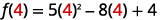
Simplify the exponents. 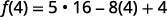
Multiply. 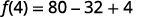
Simplify. 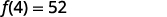
ⓑ


Simplify the exponents. 
Multiply. 
Simplify. 
ⓒ


Simplify the exponents. 
Multiply. 
For the function \(f(x)=3x^2+2x−15\), find
- \(f(3)\)
- \(f(−5)\)
- \(f(0)\).
- Answer
-
ⓐ 18 ⓑ 50 ⓒ \(−15\)
For the function \(g(x)=5x^2−x−4\), find
- \(g(−2)\)
- \(g(−1)\)
- \(g(0)\).
- Answer
-
ⓐ 20 ⓑ 2 ⓒ \(−4\)
The polynomial functions similar to the one in the next example are used in many fields to determine the height of an object at some time after it is projected into the air. The polynomial in the next function is used specifically for dropping something from 250 ft.
The polynomial function \(h(t)=−16t^2+250\) gives the height of a ball t seconds after it is dropped from a 250-foot tall building. Find the height after \(t=2\) seconds.
- Answer
-
\( \begin{array} {ll} {} &{h(t)=−16t^2+250} \\ {} &{} \\ {\text{To find }h(2)\text{, substitute }t=2.} &{h(2)=−16(2)^2+250} \\ {\text{Simplify.}} &{h(2)=−16·4+250} \\ {} &{}\\ {\text{Simplify.}} &{h(2)=−64+250} \\ {} &{} \\ {\text{Simplify.}} &{h(2)=186} \\ {} &{\text{After 2 seconds the height of the ball is 186 feet.}} \\ \end{array} \nonumber \)
The polynomial function \(h(t)=−16t^2+150\) gives the height of a stone t seconds after it is dropped from a 150-foot tall cliff. Find the height after \(t=0\) seconds (the initial height of the object).
- Answer
-
The height is \(150\) feet.
The polynomial function \(h(t)=−16t^2+175\) gives the height of a ball t seconds after it is dropped from a 175-foot tall bridge. Find the height after \(t=3\) seconds.
- Answer
-
The height is \(31\) feet.
Graph of a polynomial
We can also multiply multiple polynomials together by multiplying them similar to how we do with numbers.
For example, Multiply \((2)(3)(4)(5)=(6)(4)(5)=(24)(5)=120\).
Expand \((x-1)(x+2)(x-3)(x+4)\)
- Answer
-
Multiply the first two terms by your favorite method. \(=(x^2+x-2)(x-3)(x+4)\) Multiply the new first two \(=(x^3-2x^2-5x+6)(x+4)\) Multiply the two polynomials \(=x^4+2x^3-13x^2-14x+24\)
Let's try some more examples
Expand \((x+1)(x-1)(x+2)\)
- Answer
-
\(x^3 + 2 x^2 - x - 2\)
Expand \((x+1)(x-1)(x+2)(x-2)(x+3)\)
- Answer
-
\(x^5 + 3 x^4 - 5 x^3 - 15 x^2 + 4 x + 12\)
We saw in the first example that \((x-1)(x+2)(x-3)(x+4)=x^4+2x^3-13x^2-14x+24\). Now say we want to graph this. That is we set \(f(x)=x^4+2x^3-13x^2-14x+24\). We can graph this by plotting points but first let's evaluate this at some key points. Specifically, at 1,-2,3,-4.
We see that \(f(1)=0, f(-2)=0, f(3)=0, f(-4)=0\). Why does this make sense? Well we know that \(f(x)\) is also equal to \((x-1)(x+2)(x-3)(x+4)\) and if we plug in 1 into that we get \(f(1)=(0)(1+2)(1-3)(1+4)=0\) since 0 times anything is 0. We can see the same thing for \(f(-2),f(3)\) and \(f(-4)\). So the zeros (or x-intercept) for the function are 1,-2,3, and -4.
What about the y-intercept? Well the y-int is when x is 0 so \(f(0)=(0)^4+2(0)^3-13(0)^2-14(0)+24=24\) alternatively we can get it with the non-expanded polynomial, that is, \(f(0)=(0-1)(0+2)(0-3)(0+4)=(-1)(2)(-3)(4)=24)\).
Indeed, the graph for this function is
(x%252B2)(x-3)(x%252B4).png?revision=1&size=bestfit&width=334&height=483)
We can also go backwards by observing the zeros in the following example.
Find the polynomial that makes this graph.
(x%252B2)(x-3)(x%252B4).png?revision=1&size=bestfit&width=255&height=370)
- Answer
-
We see that -4,-2,1, and 3 are roots from the graph so that means we will have \(f(x)=(x+4)(x+2)(x-1)(x-3)\) which is just another way to write the original polynomial. We confirm that this is the right polynomial by setting x=0 to get \(f(0)=24\) which is indeed the y-int.
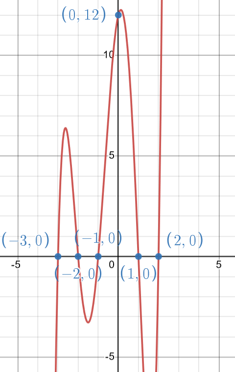
Find the polynomial that makes this graph.
(x-1)(x%252B2).png?revision=1&size=bestfit&width=484&height=295)
- Answer
-
\(f(x)=(x+1)(x-1)(x+2)\)
Find the polynomial that makes this graph.
(x-1)(x%252B2)(x-2)(x%252B3).png?revision=1&size=bestfit&width=263&height=416)
- Answer
-
\(f(x)=(x+1)(x-1)(x+2)(x-2)(x+3)\)
End Behavior
We also notice a pattern with the highest degree of the polynomial and what the graph does as x goes to \(\infty\) or \(-infty\). We shall denote this by \(x\to\infty\) and \(x\to -\infty\).
Let's describe this pattern with a table. Let \(f(x)=ax^n+\ldots+b\) be some polynomial
| If n is even | if n is odd | |
| If \(a<0\) |
As \(x\to\infty\), \(f(x)\to -\infty\) As \(x\to-\infty\), \(f(x)\to -\infty\) Example: \(-2x^6+3x^4-5x^3-15x^2+4x+12\)
|
As \(x\to\infty\), \(f(x)\to -\infty\) As \(x\to-\infty\), \(f(x)\to \infty\) Example: \(-2x^5+3x^4-5x^3-15x^2+4x+12\)
|
| If \(a>0\) |
As \(x\to\infty\), \(f(x)\to \infty\) As \(x\to-\infty\), \(f(x)\to \infty\) Example:\(2x^6+3x^4-5x^3-15x^2+4x+12\)
|
As \(x\to\infty\), \(f(x)\to \infty\) As \(x\to-\infty\), \(f(x)\to -\infty\) Example: \(-2x^5+3x^4-5x^3-15x^2+4x+12\)
|


We see this is true by plugging in values of x that are very large and very small, like 1,000,000 or -1,000,000. and seeing what the polynomial gives us.
The reason why we only pay attention to the biggest power when looking at end behavior is because all other powers become quite small in comparison. For example \((1,000,000)^5\) is much larger than \((1,000,000)^4\).
Find end behavior of
\(f(x)=8x^7-4x+5\)
Solution
The leading coefficient is positive and the highest power is an odd number, so
As \(x\to\infty\), \(f(x)\to \infty\)
As \(x\to-\infty\), \(f(x)\to \infty\)
Find end behavior of
\(f(x)=-90x^6-4x+5\)
- Answer
-
As \(x\to\infty\), \(f(x)\to -\infty\)
As \(x\to-\infty\), \(f(x)\to -\infty\)
Find end behavior of
\(f(x)=53x^{99}-7000x^{98}+5\)
- Answer
-
As \(x\to\infty\), \(f(x)\to \infty\)
As \(x\to-\infty\), \(f(x)\to -\infty\)
Find end behavior of
\(f(x)=x+5\)
- Answer
-
As \(x\to\infty\), \(f(x)\to \infty\)
As \(x\to-\infty\), \(f(x)\to -\infty\)