3.2E: Exercises for Section 3.1
- Last updated
- Save as PDF
- Page ID
- 90145
For exercises 1 - 10, use the equation \( m_{\text{sec}}=\dfrac{f(x)−f(a)}{x−a} \) to find the slope of the secant line between the values \(x_1\) and \(x_2\) for each function \(y=f(x)\).
1) \(f(x)=4x+7; \quad x_1=2, \quad x_2=5\)
- Answer
- \(m_{\text{sec}}=4\)
2) \(f(x)=8x−3;\quad x_1=−1,\quad x_2=3\)
3) \(f(x)=x^2+2x+1;\quad x_1=3,\quad x_2=3.5\)
- Answer
- \(m_{\text{sec}}=8.5\)
4) \(f(x)=−x^2+x+2;\quad x_1=0.5,\quad x_2=1.5\)
5) \(f(x)=\dfrac{4}{3x−1};\quad x_1=1,\quad x_2=3\)
- Answer
- \(m_{\text{sec}}=−\frac{3}{4}\)
6) \(f(x)=\dfrac{x−7}{2x+1};\quad x_1=−2,\quad x_2=0\)
7) \(f(x)=\sqrt{x};\quad x_1=1,\quad x_2=16\)
- Answer
- \(m_{\text{sec}}=0.2\)
8) \(f(x)=\sqrt{x−9};\quad x_1=10,\quad x_2=13\)
9) \(f(x)=x^{1/3}+1;\quad x_1=0,\quad x_2=8\)
- Answer
- \(m_{\text{sec}}=0.25\)
10) \(f(x)=6x^{2/3}+2x^{1/3};\quad x_1=1,\quad x_2=27\)
For the functions in exercises 11 - 20,
a. use the equation \( \displaystyle m_{\text{tan}}=\lim_{h→0}\frac{f(a+h)−f(a)}{h} \) to find the slope of the tangent line \(m_{\text{tan}}=f′(a)\), and
b. find the equation of the tangent line to \(f\) at \(x=a\).
11) \(f(x)=3−4x, \quad a=2\)
- Answer
- a. \(m_{\text{tan}}=−4\)
b. \(y=−4x+3\)
12) \(f(x)=\dfrac{x}{5}+6, \quad a=−1\)
13) \(f(x)=x^2+x, \quad a=1\)
- Answer
- a. \(m_{\text{tan}}=3\)
b. \(y=3x−1\)
14) \(f(x)=1−x−x^2, \quad a=0\)
15) \(f(x)=\dfrac{7}{x}, \quad a=3\)
- Answer
- a. \(m_{\text{tan}}=\frac{−7}{9}\)
b. \(y=\frac{−7}{9}x+\frac{14}{3}\)
16) \(f(x)=\sqrt{x+8}, \quad a=1\)
17) \(f(x)=2−3x^2, \quad a=−2\)
- Answer
- a. \(m_{\text{tan}}=12\)
b. \(y=12x+14\)
18) \(f(x)=\dfrac{−3}{x−1}, \quad a=4\)
19) \(f(x)=\dfrac{2}{x+3}, \quad a=−4\)
- Answer
- a. \(m_{\text{tan}}=−2\)
b. \(y=−2x−10\)
20) \(f(x)=\dfrac{3}{x^2}, \quad a=3\)
For the functions \(y=f(x)\) in exercises 21 - 30, find \(f′(a)\) using the equation \( \displaystyle f′(a)=\lim_{x→a}\frac{f(x)−f(a)}{x−a} \).
21) \(f(x)=5x+4, \quad a=−1\)
- Answer
- \(f'(-1) = 5\)
22) \(f(x)=−7x+1, \quad a=3\)
23) \(f(x)=x^2+9x, \quad a=2\)
- Answer
- \(f'(2) = 13\)
24) \(f(x)=3x^2−x+2, \quad a=1\)
25) \(f(x)=\sqrt{x}, \quad a=4\)
- Answer
- \(f'(4) = \frac{1}{4}\)
26) \(f(x)=\sqrt{x−2}, \quad a=6\)
27) \(f(x)=\dfrac{1}{x}, \quad a=2\)
- Answer
- \(f'(2) = −\frac{1}{4}\)
28) \(f(x)=\dfrac{1}{x−3}, \quad a=−1\)
29) \(f(x)=\dfrac{1}{x^3}, \quad a=1\)
- Answer
- \(f'(1) = -3\)
30) \(f(x)=\dfrac{1}{\sqrt{x}}, \quad a=4\)
For the following exercises, given the function \(y=f(x)\),
a. find the slope of the secant line \(PQ\) for each point \(Q(x,f(x))\) with \(x\) value given in the table.
b. Use the answers from a. to estimate the value of the slope of the tangent line at \(P\).
c. Use the answer from b. to find the equation of the tangent line to \(f\) at point \(P\).
31) [T] \(f(x)=x^2+3x+4, \quad P(1,8)\) (Round to \(6\) decimal places.)
| \(x\) | Slope \(m_{PQ}\) | \(x\) | Slope \(m_{PQ}\) |
| 1.1 | (i) | 0.9 | (vii) |
| 1.01 | (ii) | 0.99 | (viii) |
| 1.001 | (iii) | 0.999 | (ix) |
| 1.0001 | (iv) | 0.9999 | (x) |
| 1.00001 | (v) | 0.99999 | (xi) |
| 1.000001 | (vi) | 0.999999 | (xii) |
- Answer
- \(a. (i)5.100000, (ii)5.010000, (iii)5.001000, (iv)5.000100, (v)5.000010, (vi)5.000001, (vii)4.900000, (viii)4.990000, (ix)4.999000, (x)4.999900, (xi)4.999990, (x)4.999999\)
b. \(m_{\text{tan}}=5\)
c. \(y=5x+3\)
32) [T] \(f(x)=\dfrac{x+1}{x^2−1}, \quad P(0,−1)\)
| \(x\) | Slope \(m_{PQ}\) | \(x\) | Slope \(m_{PQ}\) |
| 0.1 | (i) | −0.1 | (vii) |
| 0.01 | (ii) | −0.01 | (viii) |
| 0.001 | (iii) | −0.001 | (ix) |
| 0.0001 | (iv) | −0.0001 | (x) |
| 0.00001 | (v) | −0.00001 | (xi) |
| 0.000001 | (vi) | −0.000001 | (xii) |
33) [T] \(f(x)=10e^{0.5x}, \quad P(0,10)\) (Round to \(4\) decimal places.)
| \(x\) | Slope \(m_{PQ}\) |
| −0.1 | (i) |
| −0.01 | (ii) |
| −0.001 | (iii) |
| −0.0001 | (iv) |
| −0.00001 | (v) |
| −0.000001 | (vi) |
- Answer
- a. \((i)4.8771, \;(ii)4.9875, \;(iii)4.9988, \;(iv)4.9999, \;(v)4.9999, \;(vi)4.9999 \)
b. \(m_{\text{tan}}=5\)
c. \(y=5x+10\)
34) [T] \(f(x)=\tan(x), \quad P(π,0)\)
| \(x\) | Slope \(m_{PQ}\) |
| 3.1 | (i) |
| 3.14 | (ii) |
| 3.141 | (iii) |
| 3.1415 | (iv) |
| 3.14159 | (v) |
| 3.141592 | (vi) |
[T] For the following position functions \(y=s(t)\), an object is moving along a straight line, where \(t\) is in seconds and \(s\) is in meters. Find
a. the simplified expression for the average velocity from \(t=2\) to \(t=2+h\);
b. the average velocity between \(t=2\) and \(t=2+h\), where \((i)\;h=0.1, \;(ii)\;h=0.01, \;(iii)\;h=0.001\), and \((iv)\;h=0.0001\); and
c. use the answer from a. to estimate the instantaneous velocity at \(t=2\) second.
35) \(s(t)=\frac{1}{3}t+5\)
- Answer
- a. \(\frac{1}{3}\);
b. \((i)\;\frac{1}{3}\) m/s, \((ii)\;\frac{1}{3}\) m/s, \((iii)\;\frac{1}{3}\) m/s, \((iv)\;\frac{1}{3}\) m/s;
c. \(\frac{1}{3}\) m/s
36) \(s(t)=t^2−2t\)
37) \(s(t)=2t^3+3\)
- Answer
- a. \(2(h^2+6h+12)\);
b. \((i)\;25.22\) m/s, \((ii)\; 24.12\) m/s, \((iii)\; 24.01\) m/s, \((iv)\; 24\) m/s;
c. \(24\) m/s
38) \(s(t)=\dfrac{16}{t^2}−\dfrac{4}{t}\)
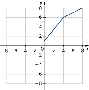
39) Use the following graph to evaluate a. \(f′(1)\) and b. \(f′(6).\)
- Answer
- a. \(1.25\); b. \(0.5\)
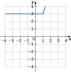
40) Use the following graph to evaluate a. \(f′(−3)\) and b. \(f′(1.5)\).
For the following exercises, use the limit definition of derivative to show that the derivative does not exist at \(x=a\) for each of the given functions.
41) \(f(x)=x^{1/3}, \quad x=0\)
- Answer
- \(\displaystyle \lim_{x→0^−}\frac{x^{1/3}−0}{x−0}=\lim_{x→0^−}\frac{1}{x^{2/3}}=∞\)
42) \(f(x)=x^{2/3}, \quad x=0\)
43) \(f(x)=\begin{cases}1, & \text{if } x<1\\x, & \text{if } x≥1\end{cases}, \quad x=1\)
- Answer
- \(\displaystyle \lim_{x→1^−}\frac{1−1}{x−1}=0≠1=\lim_{x→1^+}\frac{x−1}{x−1}\)
44) \(f(x)=\dfrac{|x|}{x}, \quad x=0\)
45) [T] The position in feet of a race car along a straight track after \(t\) seconds is modeled by the function \(s(t)=8t^2−\frac{1}{16}t^3.\)
a. Find the average velocity of the vehicle over the following time intervals to four decimal places:
i. [\(4, 4.1\)]
ii. [\(4, 4.01\)]
iii. [\(4, 4.001\)]
iv. [\(4, 4.0001\)]
b. Use a. to draw a conclusion about the instantaneous velocity of the vehicle at \(t=4\) seconds.
- Answer
- a. \((i)61.7244 ft/s, \;(ii)61.0725 ft/s, \;(iii)61.0072 ft/s, \;(iv)61.0007 ft/s\)
b. At \(4\) seconds the race car is traveling at a rate/velocity of \(61\) ft/s.
46) [T] The distance in feet that a ball rolls down an incline is modeled by the function \(s(t)=14t^2\),
where t is seconds after the ball begins rolling.
a. Find the average velocity of the ball over the following time intervals:
i. [5, 5.1]
ii. [5, 5.01]
iii. [5, 5.001]
iv. [5, 5.0001]
b. Use the answers from a. to draw a conclusion about the instantaneous velocity of the ball at \(t=5\) seconds.
47) Two vehicles start out traveling side by side along a straight road. Their position functions, shown in the following graph, are given by \(s=f(t)\) and \(s=g(t)\), where s is measured in feet and t is measured in seconds.
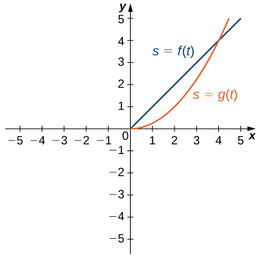
a. Which vehicle has traveled farther at \(t=2\) seconds?
b. What is the approximate velocity of each vehicle at \(t=3\) seconds?
c. Which vehicle is traveling faster at \(t=4\) seconds?
d. What is true about the positions of the vehicles at \(t=4\) seconds?
- Answer
- a. The vehicle represented by \(f(t)\), because it has traveled \(2\) feet, whereas \(g(t)\) has traveled \(1\) foot.
b. The velocity of \(f(t)\) is constant at \(1\) ft/s, while the velocity of \(g(t)\) is approximately \(2\) ft/s.
c. The vehicle represented by \(g(t)\), with a velocity of approximately \(4\) ft/s.
d. Both have traveled \(4\) feet in \(4\) seconds.
48) [T] The total cost \(C(x)\), in hundreds of dollars, to produce \(x\) jars of mayonnaise is given by \(C(x)=0.000003x^3+4x+300\).
a. Calculate the average cost per jar over the following intervals:
i. [100, 100.1]
ii. [100, 100.01]
iii. [100, 100.001]
iv. [100, 100.0001]
b. Use the answers from a. to estimate the average cost to produce \(100\) jars of mayonnaise.
49) [T] For the function \(f(x)=x^3−2x^2−11x+12\), do the following.
a. Use a graphing calculator to graph \(f\) in an appropriate viewing window.
b. Use the ZOOM feature on the calculator to approximate the two values of \(x=a\) for which \(m_{tan}=f′(a)=0\).
- Answer
-
a.
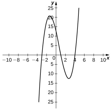
b. \(a≈−1.361,\;2.694\)
50) [T] For the function \(f(x)=\dfrac{x}{1+x^2}\), do the following.
a. Use a graphing calculator to graph \(f\) in an appropriate viewing window.
b. Use the ZOOM feature on the calculator to approximate the values of \(x=a\) for which \(m_{\text{tan}}=f′(a)=0\).
51) Suppose that \(N(x)\) computes the number of gallons of gas used by a vehicle traveling \(x\) miles. Suppose the vehicle gets \(30\) mpg.
a. Find a mathematical expression for \(N(x)\).
b. What is \(N(100)\)? Explain the physical meaning.
c. What is \(N′(100)\)? Explain the physical meaning.
- Answer
- a. \(N(x)=\dfrac{x}{30}\)
b. ∼\(3.3\) gallons. When the vehicle travels \(100\) miles, it has used \(3.3\) gallons of gas.
c. \(\frac{1}{30}\). The rate of gas consumption in gallons per mile that the vehicle is achieving after having traveled \(100\) miles.
52) [T] For the function \(f(x)=x^4−5x^2+4\), do the following.
a. Use a graphing calculator to graph \(f\) in an appropriate viewing window.
b. Use the \(nDeriv\) function, which numerically finds the derivative, on a graphing calculator to estimate \(f′(−2),\;f′(−0.5),\;f′(1.7)\), and \(f′(2.718)\).
53) [T] For the function \(f(x)=\dfrac{x^2}{x^2+1}\), do the following.
a. Use a graphing calculator to graph \(f\) in an appropriate viewing window.
b. Use the \(nDeriv\) function on a graphing calculator to find \(f′(−4),\;f′(−2),\;f′(2)\), and \(f′(4)\).
- Answer
-
a.
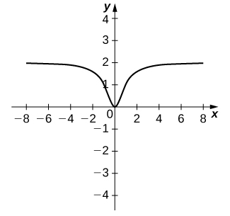
b. \(−0.028,−0.16,0.16,0.028\)

