Mathematics LibreTexts

3.10E: Exercises for Section 3.9

  • Page ID
    90161
  • \( \newcommand{\vecs}[1]{\overset { \scriptstyle \rightharpoonup} {\mathbf{#1}} } \)

    \( \newcommand{\vecd}[1]{\overset{-\!-\!\rightharpoonup}{\vphantom{a}\smash {#1}}} \)

    \( \newcommand{\id}{\mathrm{id}}\) \( \newcommand{\Span}{\mathrm{span}}\)

    ( \newcommand{\kernel}{\mathrm{null}\,}\) \( \newcommand{\range}{\mathrm{range}\,}\)

    \( \newcommand{\RealPart}{\mathrm{Re}}\) \( \newcommand{\ImaginaryPart}{\mathrm{Im}}\)

    \( \newcommand{\Argument}{\mathrm{Arg}}\) \( \newcommand{\norm}[1]{\| #1 \|}\)

    \( \newcommand{\inner}[2]{\langle #1, #2 \rangle}\)

    \( \newcommand{\Span}{\mathrm{span}}\)

    \( \newcommand{\id}{\mathrm{id}}\)

    \( \newcommand{\Span}{\mathrm{span}}\)

    \( \newcommand{\kernel}{\mathrm{null}\,}\)

    \( \newcommand{\range}{\mathrm{range}\,}\)

    \( \newcommand{\RealPart}{\mathrm{Re}}\)

    \( \newcommand{\ImaginaryPart}{\mathrm{Im}}\)

    \( \newcommand{\Argument}{\mathrm{Arg}}\)

    \( \newcommand{\norm}[1]{\| #1 \|}\)

    \( \newcommand{\inner}[2]{\langle #1, #2 \rangle}\)

    \( \newcommand{\Span}{\mathrm{span}}\) \( \newcommand{\AA}{\unicode[.8,0]{x212B}}\)

    \( \newcommand{\vectorA}[1]{\vec{#1}}      % arrow\)

    \( \newcommand{\vectorAt}[1]{\vec{\text{#1}}}      % arrow\)

    \( \newcommand{\vectorB}[1]{\overset { \scriptstyle \rightharpoonup} {\mathbf{#1}} } \)

    \( \newcommand{\vectorC}[1]{\textbf{#1}} \)

    \( \newcommand{\vectorD}[1]{\overrightarrow{#1}} \)

    \( \newcommand{\vectorDt}[1]{\overrightarrow{\text{#1}}} \)

    \( \newcommand{\vectE}[1]{\overset{-\!-\!\rightharpoonup}{\vphantom{a}\smash{\mathbf {#1}}}} \)

    \( \newcommand{\vecs}[1]{\overset { \scriptstyle \rightharpoonup} {\mathbf{#1}} } \)

    \( \newcommand{\vecd}[1]{\overset{-\!-\!\rightharpoonup}{\vphantom{a}\smash {#1}}} \)

    \(\newcommand{\avec}{\mathbf a}\) \(\newcommand{\bvec}{\mathbf b}\) \(\newcommand{\cvec}{\mathbf c}\) \(\newcommand{\dvec}{\mathbf d}\) \(\newcommand{\dtil}{\widetilde{\mathbf d}}\) \(\newcommand{\evec}{\mathbf e}\) \(\newcommand{\fvec}{\mathbf f}\) \(\newcommand{\nvec}{\mathbf n}\) \(\newcommand{\pvec}{\mathbf p}\) \(\newcommand{\qvec}{\mathbf q}\) \(\newcommand{\svec}{\mathbf s}\) \(\newcommand{\tvec}{\mathbf t}\) \(\newcommand{\uvec}{\mathbf u}\) \(\newcommand{\vvec}{\mathbf v}\) \(\newcommand{\wvec}{\mathbf w}\) \(\newcommand{\xvec}{\mathbf x}\) \(\newcommand{\yvec}{\mathbf y}\) \(\newcommand{\zvec}{\mathbf z}\) \(\newcommand{\rvec}{\mathbf r}\) \(\newcommand{\mvec}{\mathbf m}\) \(\newcommand{\zerovec}{\mathbf 0}\) \(\newcommand{\onevec}{\mathbf 1}\) \(\newcommand{\real}{\mathbb R}\) \(\newcommand{\twovec}[2]{\left[\begin{array}{r}#1 \\ #2 \end{array}\right]}\) \(\newcommand{\ctwovec}[2]{\left[\begin{array}{c}#1 \\ #2 \end{array}\right]}\) \(\newcommand{\threevec}[3]{\left[\begin{array}{r}#1 \\ #2 \\ #3 \end{array}\right]}\) \(\newcommand{\cthreevec}[3]{\left[\begin{array}{c}#1 \\ #2 \\ #3 \end{array}\right]}\) \(\newcommand{\fourvec}[4]{\left[\begin{array}{r}#1 \\ #2 \\ #3 \\ #4 \end{array}\right]}\) \(\newcommand{\cfourvec}[4]{\left[\begin{array}{c}#1 \\ #2 \\ #3 \\ #4 \end{array}\right]}\) \(\newcommand{\fivevec}[5]{\left[\begin{array}{r}#1 \\ #2 \\ #3 \\ #4 \\ #5 \\ \end{array}\right]}\) \(\newcommand{\cfivevec}[5]{\left[\begin{array}{c}#1 \\ #2 \\ #3 \\ #4 \\ #5 \\ \end{array}\right]}\) \(\newcommand{\mattwo}[4]{\left[\begin{array}{rr}#1 \amp #2 \\ #3 \amp #4 \\ \end{array}\right]}\) \(\newcommand{\laspan}[1]{\text{Span}\{#1\}}\) \(\newcommand{\bcal}{\cal B}\) \(\newcommand{\ccal}{\cal C}\) \(\newcommand{\scal}{\cal S}\) \(\newcommand{\wcal}{\cal W}\) \(\newcommand{\ecal}{\cal E}\) \(\newcommand{\coords}[2]{\left\{#1\right\}_{#2}}\) \(\newcommand{\gray}[1]{\color{gray}{#1}}\) \(\newcommand{\lgray}[1]{\color{lightgray}{#1}}\) \(\newcommand{\rank}{\operatorname{rank}}\) \(\newcommand{\row}{\text{Row}}\) \(\newcommand{\col}{\text{Col}}\) \(\renewcommand{\row}{\text{Row}}\) \(\newcommand{\nul}{\text{Nul}}\) \(\newcommand{\var}{\text{Var}}\) \(\newcommand{\corr}{\text{corr}}\) \(\newcommand{\len}[1]{\left|#1\right|}\) \(\newcommand{\bbar}{\overline{\bvec}}\) \(\newcommand{\bhat}{\widehat{\bvec}}\) \(\newcommand{\bperp}{\bvec^\perp}\) \(\newcommand{\xhat}{\widehat{\xvec}}\) \(\newcommand{\vhat}{\widehat{\vvec}}\) \(\newcommand{\uhat}{\widehat{\uvec}}\) \(\newcommand{\what}{\widehat{\wvec}}\) \(\newcommand{\Sighat}{\widehat{\Sigma}}\) \(\newcommand{\lt}{<}\) \(\newcommand{\gt}{>}\) \(\newcommand{\amp}{&}\) \(\definecolor{fillinmathshade}{gray}{0.9}\)

    In exercises 1 - 15, find \(f′(x)\) for each function.

    1) \(f(x)=x^2e^x\)

    Answer
    \(f'(x) = 2xe^x+x^2e^x\)

    2) \(f(x)=\dfrac{e^{−x}}{x}\)

    3) \(f(x)=e^{x^3\ln x}\)

    Answer
    \(f'(x) = e^{x^3\ln x}\left(3x^2\ln x+x^2\right)\)

    4) \(f(x)=\sqrt{e^{2x}+2x}\)

    5) \(f(x)=\dfrac{e^x−e^{−x}}{e^x+e^{−x}}\)

    Answer
    \(f'(x) = \dfrac{4}{(e^x+e^{−x})^2}\)

    6) \(f(x)=\dfrac{10^x}{\ln 10}\)

    7) \(f(x)=2^{4x}+4x^2\)

    Answer
    \(f'(x) = 2^{4x+2}⋅\ln 2+8x\)

    8) \(f(x)=3^{\sin 3x}\)

    9) \(f(x)=x^π⋅π^x\)

    Answer
    \(f'(x) = πx^{π−1}⋅π^x+x^π⋅π^x\ln π\)

    10) \(f(x)=\ln(4x^3+x)\)

    11) \(f(x)=\ln\sqrt{5x−7}\)

    Answer
    \(f'(x) = \dfrac{5}{2(5x−7)}\)

    12) \(f(x)=x^2\ln 9x\)

    13) \(f(x)=\log(\sec x)\)

    Answer
    \(f'(x) = \dfrac{\tan x}{\ln 10}\)

    14) \(f(x)=\log_7(6x^4+3)^5\)

    15) \(f(x)=2^x⋅\log_37^{x^2−4}\)

    Answer
    \(f'(x) = 2^x⋅\ln 2⋅\log_3 7^{x^2−4}+2^x⋅\dfrac{2x\ln 7}{\ln 3}\)

    For exercises 16 - 23, use logarithmic differentiation to find \(\dfrac{dy}{dx}\).

    16) \(y=x^{\sqrt{x}}\)

    17) \(y=(\sin 2x)^{4x}\)

    Answer
    \(\dfrac{dy}{dx} = (\sin 2x)^{4x}\big[4⋅\ln(\sin 2x)+8x⋅\cot 2x\big]\)

    18) \(y=(\ln x)^{\ln x}\)

    19) \(y=x^{\log_2x}\)

    Answer
    \(\dfrac{dy}{dx} = x^{\log_2x}⋅\dfrac{2\ln x}{x\ln 2}\)

    20) \(y=(x^2−1)^{\ln x}\)

    21) \(y=x^{\cot x}\)

    Answer
    \(\dfrac{dy}{dx} = x^{\cot x}⋅\left[−\csc^2x⋅\ln x+\dfrac{\cot x}{x}\right]\)

    22) \(y=\dfrac{x+11}{\sqrt[3]{x^2−4}}\)

    23) \(y=x^{−1/2}(x^2+3)^{2/3}(3x−4)^4\)

    Answer
    \(\dfrac{dy}{dx} = x^{−1/2}(x^2+3)^{2/3}(3x−4)^4⋅\left[\dfrac{−1}{2x}+\dfrac{4x}{3(x^2+3)}+\dfrac{12}{3x−4}\right]\)

    24) [T] Find an equation of the tangent line to the graph of \(f(x)=4xe^{(x^2−1)}\) at the point where

    \(x=−1.\) Graph both the function and the tangent line.

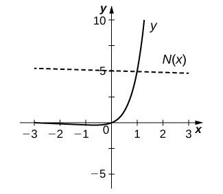
    25) [T] Find the equation of the line that is normal to the graph of \(f(x)=x⋅5^x\) at the point where \(x=1\). Graph both the function and the normal line.

    Answer
    \(y=\frac{−1}{5+5\ln 5}x+\left(5+\frac{1}{5+5\ln 5}\right)\)
    The function starts at (−3, 0), decreases slightly and then increases through the origin and increases to (1.25, 10). There is a straight line marked T(x) with slope −1/(5 + 5 ln 5) and y intercept 5 + 1/(5 + 5 ln 5).

    26) [T] Find the equation of the tangent line to the graph of \(x^3−x\ln y+y^3=2x+5\) at the point where \(x=2\). (Hint: Use implicit differentiation to find \(\dfrac{dy}{dx}\).) Graph both the curve and the tangent line.

    27) Consider the function \(y=x^{1/x}\) for \(x>0.\)

    a. Determine the points on the graph where the tangent line is horizontal.

    b. Determine the points on the graph where \(y′>0\) and those where \(y′<0\).

    Answer
    a. \(x=e \approx 2.718\)
    b. \(y'>0 \text{ for } (0,e)\) and \(y'<0 \text{ for } (e,∞).\)

    28) The formula \(I(t)=\dfrac{\sin t}{e^t}\) is the formula for a decaying alternating current.

    a. Complete the following table with the appropriate values.

    \(t\) \(\frac{\sin t}{e^t}\)
    0 (i)
    \(π/2\) (ii)
    \(π\) (iii)
    \(3π/2\) (vi)
    \(2π\) (v)
    \(2π\) (vi)
    \(3π\) (vii)

    b. Using only the values in the table, determine where the tangent line to the graph of \(I(t)\) is horizontal.

    29) [T] The population of Toledo, Ohio, in 2000 was approximately 500,000. Assume the population is increasing at a rate of 5% per year.

    a. Write the exponential function that relates the total population as a function of \(t\).

    b. Use part a. to determine the rate at which the population is increasing in \(t\) years.

    c. Use part b. to determine the rate at which the population is increasing in 10 years

    Answer
    a. \(P=500,000(1.05)^t\) individuals
    b. \(P′(t)=24395⋅(1.05)^t\) individuals per year
    c. \(39,737\) individuals per year

    30)[T] An isotope of the element erbium has a half-life of approximately 12 hours. Initially there are 9 grams of the isotope present.

    a. Write the exponential function that relates the amount of substance remaining as a function of \(t\), measured in hours.

    b. Use a. to determine the rate at which the substance is decaying in \(t\) hours.

    c. Use b. to determine the rate of decay at \(t=4\) hours.

    31) [T] The number of cases of influenza in New York City from the beginning of 1960 to the beginning of 1964 is modeled by the function \(N(t)=5.3e^{0.093t^2−0.87t},(0≤t≤4)\), where \(N(t)\) gives the number of cases (in thousands) and \(t\) is measured in years, with \(t=0\) corresponding to the beginning of 1960.

    a. Show work that evaluates \(N(0)\) and \(N(4)\). Briefly describe what these values indicate about the disease in New York City.

    b. Show work that evaluates \(N′(0)\) and \(N′(3)\). Briefly describe what these values indicate about the disease in the United States.

    Answer
    a. At the beginning of 1960 there were 5.3 thousand cases of the disease in New York City. At the beginning of 1963 there were approximately 723 cases of the disease in the United States.
    b. At the beginning of 1960 the number of cases of the disease was decreasing at rate of \(−4.611\) thousand per year; at the beginning of 1963, the number of cases of the disease was decreasing at a rate of \(−0.2808\) thousand per year.

    32) [T] The relative rate of change of a differentiable function \(y=f(x)\) is given by \(\frac{100⋅f′(x)}{f(x)}%.\) One model for population growth is a Gompertz growth function, given by \(P(x)=ae^{−b⋅e^{−cx}}\) where \(a,b\), and \(c\) are constants.

    a. Find the relative rate of change formula for the generic Gompertz function.

    b. Use part a. to find the relative rate of change of a population in \(x=20\) months when \(a=204,\;b=0.0198,\) and \(c=0.15.\)

    c. Briefly interpret what the result of part b. means.

    For exercises 33 - 36, use the population of New York City from 1790 to 1860, given in the following table.

    Year since 1790 Population
    0 33,131
    10 60,515
    20 96,373
    30 123,706
    40 202,300
    50 312,710
    60 515,547
    70 813,669

    New York City Population Over TimeSource: http://en.Wikipedia.org/wiki/Largest..._United_States

    _by_population_by_decade

    33) [T] Using a computer program or a calculator, fit a growth curve to the data of the form \(p=ab^t\).

    Answer
    \(p=35741(1.045)^t\)

    34) [T] Using the exponential best fit for the data, write a table containing the derivatives evaluated at each year.

    35) [T] Using the exponential best fit for the data, write a table containing the second derivatives evaluated at each year.

    Answer
    Year since 1790 \(P"\)
    0 69.25
    10 107.5
    20 167.0
    30 259.4
    40 402.8
    50 625.5
    60 971.4
    70 1508.5

    36) [T] Using the tables of first and second derivatives and the best fit, answer the following questions:

    a. Will the model be accurate in predicting the future population of New York City? Why or why not?

    b. Estimate the population in 2010. Was the prediction correct from part a.?


    3.10E: Exercises for Section 3.9 is shared under a not declared license and was authored, remixed, and/or curated by LibreTexts.

    • Was this article helpful?