
3.8: Improper Integrals


- Last updated
- Sep 10, 2021
- Save as PDF

( \newcommand{\kernel}{\mathrm{null}\,}\)
Learning Objectives
- Evaluate an integral over an infinite interval.
- Evaluate an integral over a closed interval with an infinite discontinuity within the interval.
- Use the comparison theorem to determine whether a definite integral is convergent.
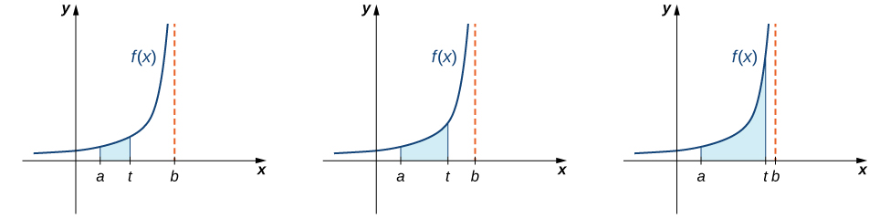
Is the area between the graph of
In this section, we define integrals over an infinite interval as well as integrals of functions containing a discontinuity on the interval. Integrals of these types are called improper integrals. We examine several techniques for evaluating improper integrals, all of which involve taking limits.
Integrating over an Infinite Interval
How should we go about defining an integral of the type
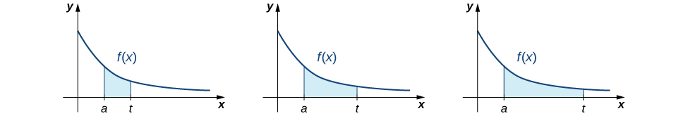
Definition: improper integral
- Let
- Let
In each case, if the limit exists, then the improper integral is said to converge. If the limit does not exist, then the improper integral is said to diverge.
- Let
In our first example, we return to the question we posed at the start of this section: Is the area between the graph of
Example
Determine whether the area between the graph of
Solution
We first do a quick sketch of the region in question, as shown in Figure
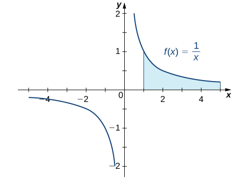
We can see that the area of this region is given by
which can be evaluated using Equation
Since the improper integral diverges to
Example
Find the volume of the solid obtained by revolving the region bounded by the graph of
Solution
The solid is shown in Figure
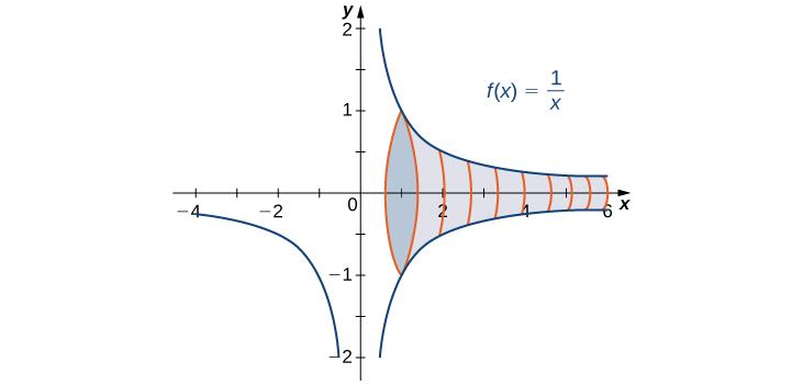
Then we have
The improper integral converges to
In conclusion, although the area of the region between the
Note: Gabriel's horn (also called Torricelli's trumpet) is a geometric figure which has infinite surface area, but finite volume. The name refers to the tradition identifying the Archangel Gabriel as the angel who blows the horn to announce Judgment Day, associating the divine, or infinite, with the finite. The properties of this figure were first studied by Italian physicist and mathematician Evangelista Torricelli in the 17th century.
Example
Suppose that at a busy intersection, traffic accidents occur at an average rate of one every three months. After residents complained, changes were made to the traffic lights at the intersection. It has now been eight months since the changes were made and there have been no accidents. Were the changes effective or is the 8-month interval without an accident a result of chance?

Probability theory tells us that if the average time between events is
where
Thus, if accidents are occurring at a rate of one every 3 months, then the probability that
where
To answer the question, we must compute
Solution
We need to calculate the probability as an improper integral:
The value
Example
Evaluate
Solution
Begin by rewriting
The improper integral converges to
Example
Evaluate
Solution
Start by splitting up the integral:
If either
Evaluate the limit. Note:
The first improper integral converges. For the second integral,
Thus,
Exercise
Evaluate
- Hint
-
- Answer
-
It converges to
Integrating a Discontinuous Integrand
Now let’s examine integrals of functions containing an infinite discontinuity in the interval over which the integration occurs. Consider an integral of the form
We use a similar approach to define
Definition: Converging and Diverging Improper Integral
- Let
- Let
- If
The following examples demonstrate the application of this definition.
Example
Evaluate
Solution
The function
The improper integral converges.
Example
Evaluate
Solution
Since
Therefore
To evaluate it, rewrite as a quotient and apply L’Hôpital’s rule.
The improper integral converges.
Example
Evaluate
Solution
Since
If either of the two integrals diverges, then the original integral diverges. Begin with
Therefore,
Exercise
Evaluate
- Hint
-
Write
- Answer
-
A Comparison Theorem
It is not always easy or even possible to evaluate an improper integral directly; however, by comparing it with another carefully chosen integral, it may be possible to determine its convergence or divergence. To see this, consider two continuous functions
for
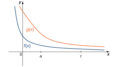
Thus, if
then
as well. That is, if the area of the region between the graph of
On the other hand, if
for some real number
must converge to some value less than or equal to
If the area of the region between the graph of
These conclusions are summarized in the following theorem.
A Comparison Theorem
Let
- If
- If
Example
Use a comparison to show that
converges.
Solution
We can see that
so if
Since
Example
Use the comparison theorem to show that
Solution
For
Exercise
Use a comparison to show that
- Hint
-
- Answer
-
Since
Laplace Transforms
In the last few chapters, we have looked at several ways to use integration for solving real-world problems. For this next project, we are going to explore a more advanced application of integration: integral transforms. Specifically, we describe the Laplace transform and some of its properties. The Laplace transform is used in engineering and physics to simplify the computations needed to solve some problems. It takes functions expressed in terms of time and transforms them to functions expressed in terms of frequency. It turns out that, in many cases, the computations needed to solve problems in the frequency domain are much simpler than those required in the time domain.
The Laplace transform is defined in terms of an integral as
Note that the input to a Laplace transform is a function of time,
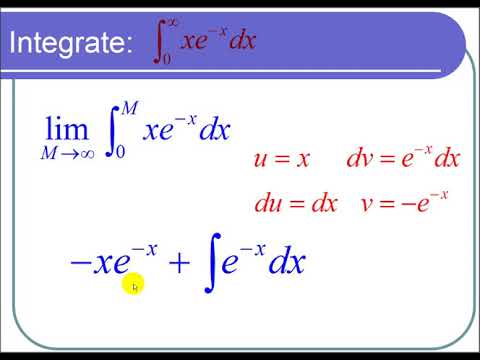
Let’s start with a simple example. Here we calculate the Laplace transform of
This is an improper integral, so we express it in terms of a limit, which gives
Now we use integration by parts to evaluate the integral. Note that we are integrating with respect to t, so we treat the variable s as a constant. We have
Then we obtain
- Calculate the Laplace transform of
- Calculate the Laplace transform of
- Calculate the Laplace transform of
Laplace transforms are often used to solve differential equations. Differential equations are not covered in detail until later in this book; but, for now, let’s look at the relationship between the Laplace transform of a function and the Laplace transform of its derivative.
Let’s start with the definition of the Laplace transform. We have
Use integration by parts to evaluate
After integrating by parts and evaluating the limit, you should see that
Then,
Thus, differentiation in the time domain simplifies to multiplication by s in the frequency domain.
The final thing we look at in this project is how the Laplace transforms of
Use integration by parts to evaluate
As you might expect, you should see that
Integration in the time domain simplifies to division by
Key Concepts
- Integrals of functions over infinite intervals are defined in terms of limits.
- Integrals of functions over an interval for which the function has a discontinuity at an endpoint may be defined in terms of limits.
- The convergence or divergence of an improper integral may be determined by comparing it with the value of an improper integral for which the convergence or divergence is known.
Key Equations
- Improper integrals
Glossary
- improper integral
- an integral over an infinite interval or an integral of a function containing an infinite discontinuity on the interval; an improper integral is defined in terms of a limit. The improper integral converges if this limit is a finite real number; otherwise, the improper integral diverges
Contributors and Attributions
Gilbert Strang (MIT) and Edwin “Jed” Herman (Harvey Mudd) with many contributing authors. This content by OpenStax is licensed with a CC-BY-SA-NC 4.0 license. Download for free at http://cnx.org.