9.6: Sequences
- Page ID
- 99788
\( \newcommand{\vecs}[1]{\overset { \scriptstyle \rightharpoonup} {\mathbf{#1}} } \)
\( \newcommand{\vecd}[1]{\overset{-\!-\!\rightharpoonup}{\vphantom{a}\smash {#1}}} \)
\( \newcommand{\dsum}{\displaystyle\sum\limits} \)
\( \newcommand{\dint}{\displaystyle\int\limits} \)
\( \newcommand{\dlim}{\displaystyle\lim\limits} \)
\( \newcommand{\id}{\mathrm{id}}\) \( \newcommand{\Span}{\mathrm{span}}\)
( \newcommand{\kernel}{\mathrm{null}\,}\) \( \newcommand{\range}{\mathrm{range}\,}\)
\( \newcommand{\RealPart}{\mathrm{Re}}\) \( \newcommand{\ImaginaryPart}{\mathrm{Im}}\)
\( \newcommand{\Argument}{\mathrm{Arg}}\) \( \newcommand{\norm}[1]{\| #1 \|}\)
\( \newcommand{\inner}[2]{\langle #1, #2 \rangle}\)
\( \newcommand{\Span}{\mathrm{span}}\)
\( \newcommand{\id}{\mathrm{id}}\)
\( \newcommand{\Span}{\mathrm{span}}\)
\( \newcommand{\kernel}{\mathrm{null}\,}\)
\( \newcommand{\range}{\mathrm{range}\,}\)
\( \newcommand{\RealPart}{\mathrm{Re}}\)
\( \newcommand{\ImaginaryPart}{\mathrm{Im}}\)
\( \newcommand{\Argument}{\mathrm{Arg}}\)
\( \newcommand{\norm}[1]{\| #1 \|}\)
\( \newcommand{\inner}[2]{\langle #1, #2 \rangle}\)
\( \newcommand{\Span}{\mathrm{span}}\) \( \newcommand{\AA}{\unicode[.8,0]{x212B}}\)
\( \newcommand{\vectorA}[1]{\vec{#1}} % arrow\)
\( \newcommand{\vectorAt}[1]{\vec{\text{#1}}} % arrow\)
\( \newcommand{\vectorB}[1]{\overset { \scriptstyle \rightharpoonup} {\mathbf{#1}} } \)
\( \newcommand{\vectorC}[1]{\textbf{#1}} \)
\( \newcommand{\vectorD}[1]{\overrightarrow{#1}} \)
\( \newcommand{\vectorDt}[1]{\overrightarrow{\text{#1}}} \)
\( \newcommand{\vectE}[1]{\overset{-\!-\!\rightharpoonup}{\vphantom{a}\smash{\mathbf {#1}}}} \)
\( \newcommand{\vecs}[1]{\overset { \scriptstyle \rightharpoonup} {\mathbf{#1}} } \)
\(\newcommand{\longvect}{\overrightarrow}\)
\( \newcommand{\vecd}[1]{\overset{-\!-\!\rightharpoonup}{\vphantom{a}\smash {#1}}} \)
\(\newcommand{\avec}{\mathbf a}\) \(\newcommand{\bvec}{\mathbf b}\) \(\newcommand{\cvec}{\mathbf c}\) \(\newcommand{\dvec}{\mathbf d}\) \(\newcommand{\dtil}{\widetilde{\mathbf d}}\) \(\newcommand{\evec}{\mathbf e}\) \(\newcommand{\fvec}{\mathbf f}\) \(\newcommand{\nvec}{\mathbf n}\) \(\newcommand{\pvec}{\mathbf p}\) \(\newcommand{\qvec}{\mathbf q}\) \(\newcommand{\svec}{\mathbf s}\) \(\newcommand{\tvec}{\mathbf t}\) \(\newcommand{\uvec}{\mathbf u}\) \(\newcommand{\vvec}{\mathbf v}\) \(\newcommand{\wvec}{\mathbf w}\) \(\newcommand{\xvec}{\mathbf x}\) \(\newcommand{\yvec}{\mathbf y}\) \(\newcommand{\zvec}{\mathbf z}\) \(\newcommand{\rvec}{\mathbf r}\) \(\newcommand{\mvec}{\mathbf m}\) \(\newcommand{\zerovec}{\mathbf 0}\) \(\newcommand{\onevec}{\mathbf 1}\) \(\newcommand{\real}{\mathbb R}\) \(\newcommand{\twovec}[2]{\left[\begin{array}{r}#1 \\ #2 \end{array}\right]}\) \(\newcommand{\ctwovec}[2]{\left[\begin{array}{c}#1 \\ #2 \end{array}\right]}\) \(\newcommand{\threevec}[3]{\left[\begin{array}{r}#1 \\ #2 \\ #3 \end{array}\right]}\) \(\newcommand{\cthreevec}[3]{\left[\begin{array}{c}#1 \\ #2 \\ #3 \end{array}\right]}\) \(\newcommand{\fourvec}[4]{\left[\begin{array}{r}#1 \\ #2 \\ #3 \\ #4 \end{array}\right]}\) \(\newcommand{\cfourvec}[4]{\left[\begin{array}{c}#1 \\ #2 \\ #3 \\ #4 \end{array}\right]}\) \(\newcommand{\fivevec}[5]{\left[\begin{array}{r}#1 \\ #2 \\ #3 \\ #4 \\ #5 \\ \end{array}\right]}\) \(\newcommand{\cfivevec}[5]{\left[\begin{array}{c}#1 \\ #2 \\ #3 \\ #4 \\ #5 \\ \end{array}\right]}\) \(\newcommand{\mattwo}[4]{\left[\begin{array}{rr}#1 \amp #2 \\ #3 \amp #4 \\ \end{array}\right]}\) \(\newcommand{\laspan}[1]{\text{Span}\{#1\}}\) \(\newcommand{\bcal}{\cal B}\) \(\newcommand{\ccal}{\cal C}\) \(\newcommand{\scal}{\cal S}\) \(\newcommand{\wcal}{\cal W}\) \(\newcommand{\ecal}{\cal E}\) \(\newcommand{\coords}[2]{\left\{#1\right\}_{#2}}\) \(\newcommand{\gray}[1]{\color{gray}{#1}}\) \(\newcommand{\lgray}[1]{\color{lightgray}{#1}}\) \(\newcommand{\rank}{\operatorname{rank}}\) \(\newcommand{\row}{\text{Row}}\) \(\newcommand{\col}{\text{Col}}\) \(\renewcommand{\row}{\text{Row}}\) \(\newcommand{\nul}{\text{Nul}}\) \(\newcommand{\var}{\text{Var}}\) \(\newcommand{\corr}{\text{corr}}\) \(\newcommand{\len}[1]{\left|#1\right|}\) \(\newcommand{\bbar}{\overline{\bvec}}\) \(\newcommand{\bhat}{\widehat{\bvec}}\) \(\newcommand{\bperp}{\bvec^\perp}\) \(\newcommand{\xhat}{\widehat{\xvec}}\) \(\newcommand{\vhat}{\widehat{\vvec}}\) \(\newcommand{\uhat}{\widehat{\uvec}}\) \(\newcommand{\what}{\widehat{\wvec}}\) \(\newcommand{\Sighat}{\widehat{\Sigma}}\) \(\newcommand{\lt}{<}\) \(\newcommand{\gt}{>}\) \(\newcommand{\amp}{&}\) \(\definecolor{fillinmathshade}{gray}{0.9}\)A sequence is a list of numbers: \(a_1 , a_2, a_3, a_4 , … , a_n, … \) A sequence can be a finite or infinite list. We call \(a_1\) the first term, \(a_2\) the second term, and \(a_n\) the “general term” or the \(n^{\text{th}}\) term. Sequences have a pattern. We describe the pattern in the general term \(a_n\).
The following sequence of numbers has a pattern you are bound to recognize:
\(2, 4, 6, 8, 10, 12, 14, 16, 18, …\)
Likely, you would describe the sequence in words: the sequence of even numbers. Alternatively, can we describe the sequence mathematically? That is, can we describe the pattern of the sequence of even numbers using a formula? Absolutely! This section will explore arithmetic sequences, how to identify them, mathematically describe their terms, and the relationship between arithmetic sequences and linear functions. Let’s get started!
For the sequence of even numbers: \(2, 4, 6, 8, 10, …\) the general term \(a_n = 2n\).

The general term \(a_n\) of a sequence is simply a function of \(n\), indicated above as \(f(n)\), where \(n\) is a natural number.
In the sequence of even numbers, what is the \(20^{\text{th}}\) term in the sequence?
Solution
The general term of the sequence of even numbers is \(a_n = 2n\). Since \(n =\) the term number, we are asked to find \(a_{20}\).
Plug in the term-number \(n=20\) into the formula \(a_n=2n\)
\(a_{20} = 2(20) = 40\)
If the sequence: \(a_1, a_2, a_3, a_4 , … , a_{n−1}, a_n, …\) exhibits a pattern such that
\[a_n − a_{n−1} = d\]
For all \(n\), then the real number \(d\) is called the common difference, and the sequence is an arithmetic sequence.
A sequence is given. If the sequence is an arithmetic sequence, give the common difference. If the sequence is not an arithmetic sequence, explain how it fails to be arithmetic.
- \(25, 32, 39, 46, 53, 60, …\)
- \(2, 4, 8, 16, 32, …\)
- \(3^2 , 3^4, 3^6, 3^8, 3^{10}, …\)
- \(0, 1, 0, 1, 0, 1, …\)
Solution
- Is the sequence
\(25, 32, 39, 46, 53, 60, … \)
an arithmetic sequence?
\(\begin{array} &a_2 − a_1 &= 32 − 25 &= \textcolor{red}{7} \\ a_3 − a_2 &= 39 − 32 &= \textcolor{red}{7} \\a_4 − a_3 &= 46 − 39 &= \textcolor{red}{7} \\a_5 − a_4 &= 53 − 46 &= \textcolor{red}{7} \\a_6 − a_5 &= 60 − 53 &= \textcolor{red}{7} \end{array}\)
The sequence is arithmetic and the common difference is \(7\).
- Is the sequence
\(2, 4, 8, 16, 32, …\)
an arithmetic sequence?
\(\begin{array} &a_2 − a_1 &= 4 − 2 &= \textcolor{red}{2} \\ a_3 − a_2 &= 8 − 4 &= \textcolor{red}{4} \\a_4 − a_3 &= 16 − 8 &= \textcolor{red}{8} \\a_5 − a_4 &= 32 − 16 &= \textcolor{red}{16} \\ &&\textcolor{red}{2 \neq 4 \neq 8 \neq 16} \end{array}\)
The sequence is not arithmetic. \(a_n − a_{n-1}\) does not yield a common difference.
- Is the sequence
\(3^2 , 3^4, 3^6, 3^8, 3^{10}, …\)
an arithmetic sequence?
\(\begin{array} &3^4 − 3^2 &= 3^2 (3^2 − 1) &= 9 \cdot 8 &= \textcolor{red}{72} \\ 3^6 − 3^4 &= 3^4 (3^2 − 1) &= 81 \cdot 8 &= \textcolor{red}{648} \end{array}\)
Since \(a_3 − a_2 \neq a_2 − a_1\), we conclude the sequence is not arithmetic.
- Is the sequence
\(0, 1, 0, 1, 0, 1, …\)
an arithmetic sequence?
\(\begin{array} 1-0 &= \textcolor{red}{1} \\ 0-1 &= \textcolor{red}{-1} \end{array}\)
Since \(a_3 − a_2 \neq a_2 − a_1\), the sequence is not arithmetic.
If a sequence is arithmetic, the general term \(a_n\) is determined using the common difference, \(d\), of the sequence. Functions of the form \(y = mx+b\), known as linear functions, have a strong relationship to arithmetic sequences. The slope \(m\) of a linear function is equivalent to the common difference \(d\) of an arithmetic sequence. Let’s compare arithmetic sequences to linear functions to build \(a_n\), the general term of an arithmetic sequence.
Find the general term \(a_n\) of each arithmetic sequence:
- \(4, 7, 10, 13, 16, …\)
- \(100, 80, 60, 40, 20, …\)
Solution
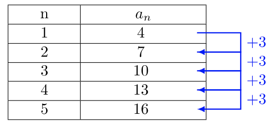
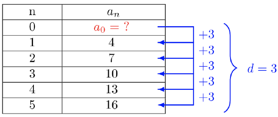
We will create a table of values for each sequence. The first column will be the term number, \(n\), starting with \(n = 1\). The second column will list the terms of the sequence. The common difference is shown on the side of the second column.
- The sequence \(4, 7, 10, 13, 16, …\) has the common difference \(d = 3\). But it’s also the slope \(m\) of the linear function \(f(x) = mx + b\).
\[m = \dfrac{a_n − a_{n-1}}{n − (n − 1))} = \dfrac{d}{1} = d\]

The above table essentially mimics any linear function, \(f(x) = mx+b\).
- Instead of \(x\), sequences use \(n\)−values.
- Instead of \(m =\) slope in linear functions, sequences use \(d =\) common difference.
- Instead of \(b\), a sequence notates the same value with \(a_0\).
If \(a_1\) denotes the first term of a sequence, then the general term of a sequence is:
\[a_n = f(n) = d \cdot n + a_0\]
To find the general term, \(a_n\), we will need to find the value \(a_0\). There are several ways to do this, but perhaps the simplest is to create an extra row where \(n = 0\), then use the common difference to find \(a_0\). The common difference pattern is maintained and \(a_0 + d = a_1\).

Find the value \(a_0\):
\(\begin{array} &&a_0 + 3 &= 4 \\&a_0 + 3 − 3 &= 4 − 3 \\&a_0 &= 1\end{array}\)
The general term of the sequence is:
\(a_n = 3n + 1\)
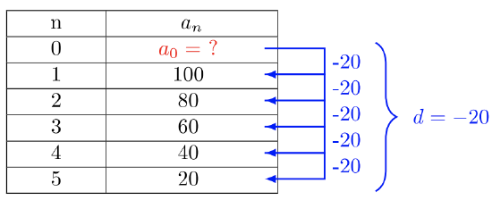
- Use the same strategy for Example \(8.1.3\)a to solve Example \(8.1.3\)b. Create a table, find the common difference, \(d\), and find the \(a_0\) term of the sequence \(100, 80, 60, 40, 20, …\)

The common difference \(d = −20\). Find the value \(a_0\).
\(\begin{array} &&a_0 − 20 &= 100 \\ &a_0 − 20 + 20 &= 100 + 20 \\ &a_0 &= 120 \end{array}\)
The general term of the sequence is:
\(a_n = −20n + 120\)
An arithmetic sequence with first term \(a_1\) and common difference \(d\) is given by \(a_{n} = a_1 + (n-1) d, \quad n \geq 1 \label{arithgeoformula} \) for \(n^{\textrm{th}}\) term.
A five-year old child receives an allowance of \($1\) each week. Their parents promise them an annual increase of \($2\) per week.
- Write a formula for the child’s weekly allowance in a given year.
- What will the child’s allowance be when he is \(16\) years old?
Solution
- The situation can be modeled by an arithmetic sequence with an initial term of \(1\) and a common difference of \(2\).
Let \(A\) be the amount of the allowance and \(n\) be the number of years after age \(5\). Using the altered explicit formula for an arithmetic sequence we get:
\(A_n=1+2n\)
- We can find the number of years since age \(5\) by subtracting.
\(16−5=11\)
We are looking for the child’s allowance after \(11\) years. Substitute \(11\) into the formula to find the child’s allowance at age \(16\).
\(A_{11}=1+2(11)=23\)
The child’s allowance at age \(16\) will be \($23\) per week.
Geometric sequences, on the other hand, have a common ratio. Each term after the first term is obtained by multiplying the previous term by \(r\), the common ratio. As an example, the following sequence does not have a common difference, so it is not an arithmetic sequence. Instead, this sequence has a common ratio, \(r\):
\(\dfrac{a_n}{a_{n−1}} = r = 2 \nonumber\)
and it is a geometric sequence:
\(2,4,8,16,32,64,128\)
Notice that each term is double the previous term. By multiplying any term by \(2\), we obtain the subsequent term. A common ratio is the hallmark signature of a geometric sequence.
If the sequence: \(a_1 , a_2, a_3, a_4 , … , a_{n−1}, a_n, …\) exhibits a pattern (\(a ≠ 0\) and \(r ≠ 0\)) such that
\(a_1, a_1r, a_1r^2 , a_1r^3 , … , a_1r^{n−1} , a_1r^n , …\)
Then the sequence is geometric and \(r\) is called the common ratio, where \(\dfrac{a_n}{a_{n-1}} = r\)
A geometric sequence is analogous to an exponential function, \(f(x) = ab^x\), where \(a\) and \(b\) are constants, \(a=\) any real number and \(b > 0\). The general term \(a_n\) for a geometric sequence will mimic the exponential function formula, but modified in the following way:
- Instead of \(x =\) any real number, the domain of the geometric sequence function is the set of natural numbers \(n\).
- The constant \(a\) will become the first term, or \(a_1\), of the geometric sequence.
- The constant \(b\) is replaced by the common ratio \(r\), but \(r\) can be positive or negative.
The geometric sequence with common ratio \(r\):
\(a_1, a_1r, a_1r^2 , a_1r^3 , … , a_1r^{n−1} , …\)
has general term
\(a_n = a_1r^{n−1}\)
The first term of the geometric sequence is \(a_1\), or \(a_1r^0\). Recall that \(r^0 = 1\).It’s worth mentioning that, in some cases, the first term is better notated as \(a_0\) rather than \(a_1\). If we use \(a_0 =\) first term (starting the sequence at \(n = 0\)), then the geometric sequence would be notated: \(a_0, a_0r, a_0r^2 , a_0r^3\), … and the general term is \(a_n = a_0r^n\). Although the term-number no longer matches the subscript (i.e. \(a_1=\) second term, \(a_2 =\) third term, etc.), the exponent on \(r\) tells us how many times \(r\) was applied. In real-life problems that have an initial value to which \(r\) is repetitively multiplied, allow yourself the flexibility to call the initial amount \(a_0\).
Determine the common ratio of the geometric sequence: \(15, 45, 135, 405, …\) and give the general term, \(a_n\). Then find the \(10^{\text{th}}\) term of the sequence, or \(a_{10}\).
Solution
Finding the common ratio is a matter of dividing any term by its previous term:
\(\dfrac{45}{15} = 3 = r\).
Therefore, the general term of the sequence is:
\(a_n = 15 \cdot 3^{n-1}\)
The general term gives us a formula to find \(a_{10}\). Plug \(n = 10\) into the general term \(a_n\).
\(a_{10} = 15 \cdot 3^{10−1} = 15 \cdot 3^9 = 295245\)
Determine the common ratio of the geometric sequence: \(8, −12, 18, −27, …\) and give the general term \(a_n\). Then find the \(7^{\text{th}}\) term of the sequence.
Solution
Notice the sequence alternates in sign value: positive, negative, positive, negative, … An alternating sequence occurs when \(r < 0\). We expect the \(r\)-value to be negative.
The common ratio is found by dividing two consecutive terms. Let’s divide \(\dfrac{a_2}{a_1}\).
\(\dfrac{−12}{8} = -\dfrac{3}{2} = -1.5 = r\)
Therefore, the general term of the sequence is:
\(a_n = -1.5 \cdot 8^{n-1}\)
The general term gives us a formula to find \(a_7\). Plug into \(n = 7\) in \(a_n\) to find the \(7^{\text{th}}\) term:
\(a_7 = 8(−1.5)^{7−1} = 8(−1.5)^6 = 91.125\)
A filtering process can reduce Chemical B by \(10\%\). The process can be repeated and have the same reduction rate of \(10\%\) each time. Initially, there is \(7\) mg of Chemical B before filtering. How much of Chemical B remains after \(4\) filtering processes? Round the answer to \(2\) decimal places.
Solution
If chemical B is reduced by \(10\%\), then \(90\%\) remains after filtering. The sequence would end after \(4\) filters. The common ratio \(r = 0.9\) and we apply this common ratio \(4\) times to the initial value, \(7\) mg:

Rather than performing each multiplication separately, it’s easier to compute the remaining quantity of Chemical B using the formula for the general term:
\(7 \cdot (0.9)^4 = 4.5927\)
Answer After \(4\) filtering processes, \(4.59\) mg of Chemical B remains.
A famous and important sequence is the Fibonacci sequence, named after the Italian mathematician known as Leonardo Pisano, whose nickname was Fibonacci, and who lived from 1170 to 1230. This sequence is: \[\{1,1,2,3,5,8,13,21,34,55, \ldots \ldots \ldots\}\] This sequence is defined recursively. This means each term is defined by the previous terms.
The Fibonacci sequence is defined by \(f_{1}=1, f_{2}=1, f_{n}=f_{n-1}+f_{n-2}\).
In other words, to get the next term in the sequence, add the two previous terms.
\(\{1, 1, 1+1=2, 2+1=3, 3+2=5, 5+3=8, 8+5=13, 13+8=21, 21+13=34, 34+21=55, 55+34=89, 89+55=144, \cdots\}\)
Find the 13th, 14th, and 15th Fibonacci numbers
Solution
First, notice that there are already 12 Fibonacci numbers listed above, so to find the next three Fibonacci numbers, we simply add the two previous terms to get the next term as the definition states.
\(f_{13}=144+89=233, f_{14}=233+144=377, f_{15}=377+233=610\)
We can find the Fibonacci numbers in all around us in nature. The number of branches on some trees or the number of petals of some daisies are often Fibonacci numbers
a. Daisy with 13 petals b. Daisy with 21 petals
a. b.
Fibonacci numbers also appear in spiral growth patterns such as the number of spirals on a cactus or in sunflowers seed beds.
a. Cactus with 13 clockwise spirals b. Sunflower with 34 clockwise spirals and 55 counterclockwise spirals
a. b.
Another interesting fact arises when looking at the ratios of consecutive Fibonacci numbers.
|
Fibonacci number |
divided by the one before |
ratio |
|---|---|---|
|
1 |
||
|
1 |
1/1 |
= 1.0000 |
|
2 |
2/1 |
= 2.0000 |
|
3 |
3/2 |
= 1.5000 |
|
5 |
5/3 |
= 1.6667 |
|
8 |
8/5 |
= 1.6000 |
|
13 |
13/8 |
= 1.6250 |
|
21 |
21/13 |
= 1.6154... |
|
34 |
34/21 |
= 1.6190... |
|
55 |
55/34 |
= 1.6177... |
|
89 |
89/55 |
= 1.6182... |
|
... |
... |
... |
|
|
= 1.6180... |
The number that these ratios are getting closer to is a special number called the Golden Ratio which is denoted by \(\phi\) (the Greek letter phi).
The Golden Ratio: \(\phi=\frac{1+\sqrt{5}}{2}\). The Golden Ratio has the decimal approximation of \(\phi=1.6180339887\).
The Golden Ratio is a special number for a variety of reasons. It is also called the divine proportion and it appears in art and architecture. It is claimed by some to be the most pleasing ratio to the eye.
If the length of a rectangle divided by its width is equal to the Golden Ratio, then the rectangle is called a golden rectangle.
 Figure \(\PageIndex{1}\): Image by Peter John Acklam is licensed by CC-3.0
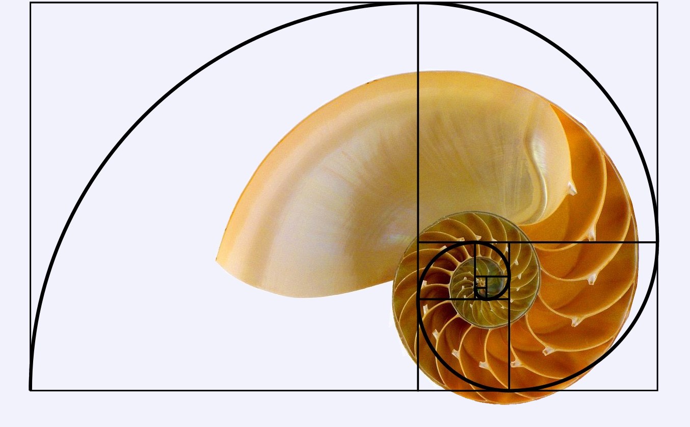
If you cut off a square on one end of the rectangle, the smaller rectangle is again a golden rectangle. If you continue doing this, and connect the opposite diagonals of the squares that you are cutting off with a smooth curve, you generate a spiral.

Here is a nautilus shell and the golden rectangle spiral on top.


