22.5: J1.05- Section 1 Part 4

Last updated
Save as PDF

Page ID: 51728

$ \newcommand{\vecs}[1]{\overset { \scriptstyle \rightharpoonup} {\mathbf{#1}} } $ $ \newcommand{\vecd}[1]{\overset{-\!-\!\rightharpoonup}{\vphantom{a}\smash {#1}}} $$\newcommand{\id}{\mathrm{id}}$ $ \newcommand{\Span}{\mathrm{span}}$ $ \newcommand{\kernel}{\mathrm{null}\,}$ $ \newcommand{\range}{\mathrm{range}\,}$ $ \newcommand{\RealPart}{\mathrm{Re}}$ $ \newcommand{\ImaginaryPart}{\mathrm{Im}}$ $ \newcommand{\Argument}{\mathrm{Arg}}$ $ \newcommand{\norm}[1]{\| #1 \|}$ $ \newcommand{\inner}[2]{\langle #1, #2 \rangle}$ $ \newcommand{\Span}{\mathrm{span}}$ $\newcommand{\id}{\mathrm{id}}$ $ \newcommand{\Span}{\mathrm{span}}$ $ \newcommand{\kernel}{\mathrm{null}\,}$ $ \newcommand{\range}{\mathrm{range}\,}$ $ \newcommand{\RealPart}{\mathrm{Re}}$ $ \newcommand{\ImaginaryPart}{\mathrm{Im}}$ $ \newcommand{\Argument}{\mathrm{Arg}}$ $ \newcommand{\norm}[1]{\| #1 \|}$ $ \newcommand{\inner}[2]{\langle #1, #2 \rangle}$ $ \newcommand{\Span}{\mathrm{span}}$$\newcommand{\AA}{\unicode[.8,0]{x212B}}$

Negative output values in exponential models: When the initial amount is a negative number (this usually happens when the y value describes a difference from a reference value), the only difference is that all of the model’s output values will be negative and the graphs will thus be reflected around the x-axis, “upside down” compared to models with positive initial values.

Relationship of exponential models with negative initial amounts to the x-axis
$graph1$	$graph2$	$graph3$	$graph4$
Exponential growth	Faster growth rate	Exponential decay	Faster decay rate

Example 5: The table to the right shows the temperature of a soda can as it warms up in a room whose temperature is 75 ° F. Use an exponential model to: [a] estimate the decay rate per minute of the difference between the can temperature and the room temperature, [b] predict the can temperature at 20 minutes, and [c] estimate the half-life of the warming process.

Solution:

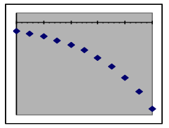
Since the temperature of the can is not converging on zero, we can’t directly use can temperature as a variable in an exponential-decay model. Instead, we will subtract the room temperature from the can temperature and use that difference as the output variable for the model.

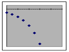
Put this dataset into the exponential-model spreadsheet, then adjust the parameters to make the model fit the data. You will find that the data is well matched by an exponential model whose initial-value parameter is -40 and whose “growth” rate is -0.09 (which is really a decay rate since it is negative).

Original data

Minutes out of cooler	Temperature of can
0	35
5	50
10	59
15	65

Redefined data

Minutes out of cooler	Degrees from 75° F
0	-40
5	-25
10	-16
15	-10

Evaluating the model for x = 20 gives a predicted difference at that time of 6.1 degrees below the room temperature of 75°F.

The data point whose y value is furthest from zero is the first one at (x=0, y=-40). The line halfway to the x-axis is at y=–20, which crosses the model graph at between 7 and 8 minutes.

Answers:

The decay rate of the temperature difference is 8.8% per minute.
The predicted temperature at 20 minutes is 68.9°F.
The half-life of the warming process is between 7 and 8 minutes.

$graph5$

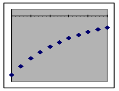
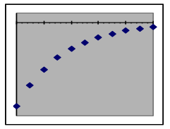
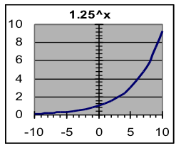
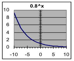
Symmetry of exponential growth and decay: Despite their different responses to large input valves (as described in the previous two paragraphs) exponential growth and decay are basically the same process, as shown by the growth and decay graphs shown to the right. These graphs are mirror images of each other, indicating that in this context growth is simply backwards decay, and vice versa.

This is why the same mathematical formula can be used for both growth and decay—the difference is just whether the base that is used is larger or smaller than 1.

$graph6$

$graph7$

Tip on fitting exponential models by hand: If you get strange results in an exponential-modeling problem, check to see if you have made the rate too large (perhaps by entering a percentage without a percent character where a decimal was expected). This causes particularly dramatic errors when a negative number is entered, since attempting to raise a negative number to a fractional power will cause the spreadsheet to show an error message.

Mathematics for Modeling. Authored by: Mary Parker and Hunter Ellinger. License: CC BY: Attribution