22.11: J1.11- Exercises

Last updated
Save as PDF

Page ID: 51723

$ \newcommand{\vecs}[1]{\overset { \scriptstyle \rightharpoonup} {\mathbf{#1}} } $ $ \newcommand{\vecd}[1]{\overset{-\!-\!\rightharpoonup}{\vphantom{a}\smash {#1}}} $$\newcommand{\id}{\mathrm{id}}$ $ \newcommand{\Span}{\mathrm{span}}$ $ \newcommand{\kernel}{\mathrm{null}\,}$ $ \newcommand{\range}{\mathrm{range}\,}$ $ \newcommand{\RealPart}{\mathrm{Re}}$ $ \newcommand{\ImaginaryPart}{\mathrm{Im}}$ $ \newcommand{\Argument}{\mathrm{Arg}}$ $ \newcommand{\norm}[1]{\| #1 \|}$ $ \newcommand{\inner}[2]{\langle #1, #2 \rangle}$ $ \newcommand{\Span}{\mathrm{span}}$ $\newcommand{\id}{\mathrm{id}}$ $ \newcommand{\Span}{\mathrm{span}}$ $ \newcommand{\kernel}{\mathrm{null}\,}$ $ \newcommand{\range}{\mathrm{range}\,}$ $ \newcommand{\RealPart}{\mathrm{Re}}$ $ \newcommand{\ImaginaryPart}{\mathrm{Im}}$ $ \newcommand{\Argument}{\mathrm{Arg}}$ $ \newcommand{\norm}[1]{\| #1 \|}$ $ \newcommand{\inner}[2]{\langle #1, #2 \rangle}$ $ \newcommand{\Span}{\mathrm{span}}$$\newcommand{\AA}{\unicode[.8,0]{x212B}}$

Part I.

Reproduce the results in Examples 1–10.

Part II.

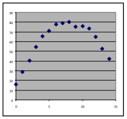
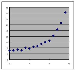
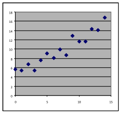
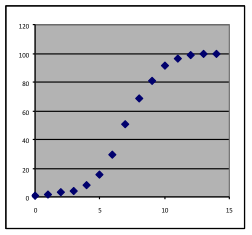
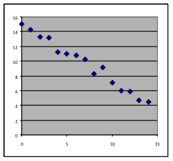
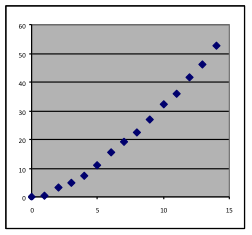
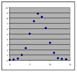
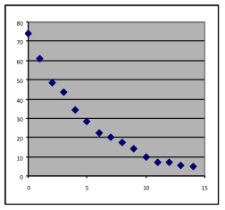
11 & 12. For each of the graphs below, identify where a linear, quadratic, or exponential model would be appropriate, or where none of these three choices would work. In each case, write a sentence stating what reason you have for the choice you make.

[11a]

[11b]

[11c]

[11d]

[12a]

[12b]

[12c]

[12d]

For each dataset in the following problems, please do not type it in yourself, but find the data table shown below on the course web page and “copy and paste” it into the spreadsheet. This will save you quite a lot of work.

Instructions on using modeling spreadsheets to build best-fit models (for use on exercises 13-20):

Copy the data into the Data Scratch Pad worksheet in Models.xls and make a scatter plot to look at to decide what kind of formula (linear, quadratic, or exponential) to use for the model.
Copy the Models.xls template designed to fit the chosen kind of model into a new worksheet, labeling the new worksheet with a reference to the problem.
Copy the data into the worksheet, putting the input data values in column A and the output data values in column B, with the numbers starting at line 3.
Select C3:E3, then spread the formulas in these cells down to all the rows that have data values.
Make a scatter-plot of columns A to C, which should give you a graph of the data in one color combined with a graph of the model values in a different color.
Adjust the parameters until the model graph is as close to the data as possible, indicating that the current parameter settings for the chosen model fit the data about as well as a model of that kind can.
Examine the graph to see whether this is a good model (the data points are randomly above and below the model) or whether a better model should be looked for.

Drug concentrations
Elapsed hours	Concentration (mg/ml)
1	17.4
2	11.2
3	7.5
4	4.7
5	3.2
6	2.1

Coffee cool-off in 70º room
Minutes since pouring	Coffee temp. °F
0	112.7
2	103.6
4	96.8
6	91.2
8	86.7
10	83.3

Number of web sites
Month/Year	Sites
June 1993	130
Dec 1993	623
June 1994	2,738
Dec 1994	10,022
June 1995	23,500
Dec 1995	92,000

World Population Growth
Year	Population
1900	1,550,000
1910	1,750,000
1920	1,860,000
1930	2,070,000
1940	2,300,000
1950	2,400,000

Stopping Distances
Speed (mph)	Distance (feet)
20	41
30	71
40	118
50	176
60	240
70	316

UT Austin Tuition
Year	Tuition
1989	410
1990	440
1991	510
1992	590
1993	715
1994	770
1995	930
1996	1,085
1997	1,200

The concentration of a drug in the bloodstream is measured hourly after injection, giving the results shown in the “Drug Concentrations” dataset above:
1. Identify the input and output variables.
2. Use a spreadsheet to make an appropriate graph and label the axes. (hand-labeling is okay)
3. Use the exponential-model spreadsheet to find a good exponential model and state its equation.
4. Using the model, predict the concentration at 9 hours.
5. How long after the injection does the model predict that the concentration will have fallen to 10.0 mg/ml?
6. What decay rate does the model imply for the concentration of the drug?
The temperature of a cup of coffee is measured every 2 minutes, giving the “Coffee cool-off” dataset shown above. The room temperature is 70° F.
1. Identify the input and output variables.
2. Restate the temperatures into a form suitable for an exponential model.
3. Use a spreadsheet to make an appropriate graph and label the axes. (hand-labeling is okay)
4. Use the exponential-model spreadsheet to find a good exponential model for the temperature difference and state its equation.
5. What decay rate does the model imply for the temperature difference?
6. Using the model, predict the temperature 15 minutes after pouring.
7. About how long after pouring will the temperature be 80° F?
Solve the previous exercise by modifying the model formula rather than restating the temperatures.
The number of web sites grew rapidly once the world wide web was invented in 1993. Use the “Number of web sites” dataset above to:
1. Identify the input and output variables.
2. Restate the date variable in months since January 1993.
3. Use a spreadsheet to make an appropriate graph and label the axes. (hand-labeling is okay)
4. Use the exponential-model spreadsheet to find an exponential model that fits the data well and state its equation.
5. State the growth rate per month implied by this model.
6. How many web sites does this model predict for Dec 1997?
The population of the world for the first six decades of the twentieth century is given in the “World Population Growth” dataset above.
1. Identify the input and output variables.
2. Modify the data to restate the date variable in years since 1900.
3. Use a spreadsheet to make an appropriate graph and label the axes. (hand-labeling is okay)
4. Use the exponential-model spreadsheet to find an exponential model that fits the data well and state its equation.
5. State the growth rate per year implied by this model.
6. What world population does this model predict for 2000?
Solve the previous exercise by modifying the model formula rather than restating the date variable.
For the “Stopping Distances” dataset above giving the stopping distance of a car at various speeds,
1. Identify the input and output variables.
2. Fit an exponential model to the data and state the model formula.
3. Fit a quadratic model to the data and state the model formula.
4. Which model better fits the data? How can you tell?
5. Use the better model to predict the stopping distance at 80 mph.
6. What stopping distance does the model predict for zero mph? Does this prediction make sense?
For the “UT Austin Tuition” dataset shown above,
1. Identify the input and output variables.
2. Fit a linear model to the data and state the model formula.
3. Use the linear model to predict 2006 tuition.
4. Fit an exponential model to the data and state the model formula.
5. Use the exponential model to predict 2006 tuition.
6. State which model you think is better for the tuition dataset, and what arguments you could make to convince someone else that your conclusion is correct.
What percentage growth or decay rate is implied by these exponential models?
1. y = 443.2 × (1.07)x
2. y = 0.134 × (1.025)x
3. y = 5.3 × (0.97)x
What percentage growth or decay rate is implied by these exponential models?
1. y = 3.52 × (0.94)x
2. y = 69 × (1.11)x
3. y = 0.825 × (1.075)x
What prediction does the model y = 3.52 × (0.94)x make for:
1. x = 10
2. x = 3.178
3. x = 0
What prediction does the model 443.2 × (1.07)x make for:
1. x = 10
2. x = 3.178
3. x = 0

Mathematics for Modeling. Authored by: Mary Parker and Hunter Ellinger. License: CC BY: Attribution