25.1: O.01- Overview

Last updated
Save as PDF

Page ID: 51753

$ \newcommand{\vecs}[1]{\overset { \scriptstyle \rightharpoonup} {\mathbf{#1}} } $ $ \newcommand{\vecd}[1]{\overset{-\!-\!\rightharpoonup}{\vphantom{a}\smash {#1}}} $$\newcommand{\id}{\mathrm{id}}$ $ \newcommand{\Span}{\mathrm{span}}$ $ \newcommand{\kernel}{\mathrm{null}\,}$ $ \newcommand{\range}{\mathrm{range}\,}$ $ \newcommand{\RealPart}{\mathrm{Re}}$ $ \newcommand{\ImaginaryPart}{\mathrm{Im}}$ $ \newcommand{\Argument}{\mathrm{Arg}}$ $ \newcommand{\norm}[1]{\| #1 \|}$ $ \newcommand{\inner}[2]{\langle #1, #2 \rangle}$ $ \newcommand{\Span}{\mathrm{span}}$ $\newcommand{\id}{\mathrm{id}}$ $ \newcommand{\Span}{\mathrm{span}}$ $ \newcommand{\kernel}{\mathrm{null}\,}$ $ \newcommand{\range}{\mathrm{range}\,}$ $ \newcommand{\RealPart}{\mathrm{Re}}$ $ \newcommand{\ImaginaryPart}{\mathrm{Im}}$ $ \newcommand{\Argument}{\mathrm{Arg}}$ $ \newcommand{\norm}[1]{\| #1 \|}$ $ \newcommand{\inner}[2]{\langle #1, #2 \rangle}$ $ \newcommand{\Span}{\mathrm{span}}$$\newcommand{\AA}{\unicode[.8,0]{x212B}}$

Modeling, Part VI. Combining Modeling Formulas

Objectives:

Be able to make and use compound models, in which two basic models are added together.
Detect and avoid confounding of parameters in compound models.
Construct and use composite models by combining formulas with IF, MAX, or MIN functions.
Use compound or composite models to separate different effects reflected in a dataset.

Overview

Combining models by addition:

Nine different kinds of basic models have been discussed in this course so far: constant average, linear, quadratic, exponential, logistic, normal, sinusoidal, power and logarithmic functions. Each reflects a particular type of relationship that frequently occurs between two variables. Thus often the best-fit settings of one of these basic models will fully match a measurement set, except for random noise.

But sometimes more than one type of process significantly influences the relationship between two variables. In such cases, combining two or more basic models is needed to provide a formula that fits the data well. This increases the number of model parameters, but the automated fitting that Solver supplies makes it almost as easy to fit a six-parameter combined model as a two-parameter basic model.

Most often the combination is just the sum of two basic model formulas (such as an exponential model plus a baseline value, as would be appropriate to model the temperature of an object cooling off to an unknown room temperature). It may even be useful to combine two models of the same type but with different parameter settings – a model of outdoor temperature might consist of one sinusoid with a one-day wavelength (matched to day/night effects) added to another sinusoid with a one-year wavelength (reflecting seasonal changes). Occasionally what is needed for a good fit is more complicated, such as when the output of one basic model is used as the input to another type of model.

Examples of compound models, formed by addition of two basic models
$123.png$	$212.png$

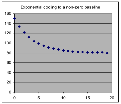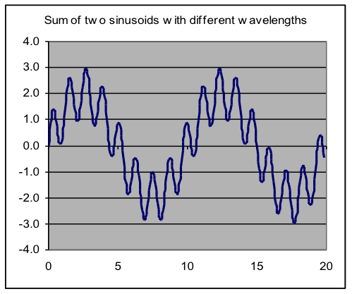The main potential difficulty that can arise from combining models is that sometimes particular parameters in the two models control the same thing (e.g., vertical offset), a situation called confounding. When Solver searches for a fit in such a case, it is unpredictable which of these parameters it will change, or what final values they will reach. The solution to this difficulty is to drop one of the parameters from the compound model – which one is usually obvious when the meaning of the parameters is considered.

Combining models by composition (using different models for different ranges of input values):

Sometimes a relationship between two variables matches different formulas for different parts of the range of input values. One way this may be modeled in a spreadsheet is by using the different formulas with the IF function – for example, if C3 contains “=IF(A3>100,400*A3,4*A3^2)”, the model function will change from linear to quadratic for values of x greater than 100. In a real modeling formula, the two formulas used in the IF function would also include parameter references such as $G$3 and $G$4. If the transition point is not known from the problem, it can be made a parameter, and thus deduced from the data (such a formula might begin “=IF(A3>$G$3,…” ).

Another way that different formulas can be used in different regions is to use the MAX (or MIN) functions so that the larger (or smaller) result of two formulas is used. This is often appropriate in situations where two separate processes are acting to limit the relationship. An example is the speed of a car as it brakes to a stop as fast as it can, where the rate of deceleration is limited by whichever of two effects is smaller: the friction of the tires with the road, and how much heat the brakes can dissipate.

Examples of composite models, formed by using different model formulas for different input ranges
$37.png$	$45.png$

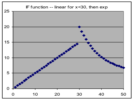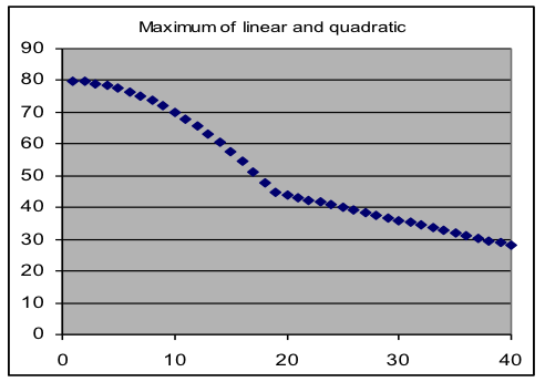An abrupt change in slope or value in graphs of models produced by these composition methods generally makes it obvious where the model switches from one formula to the other.

Mathematics for Modeling. Authored by: Mary Parker and Hunter Ellinger. License: CC BY: Attribution