21.7: I1.07- Section 5 Part 1

Last updated
Save as PDF

Page ID: 51719

$ \newcommand{\vecs}[1]{\overset { \scriptstyle \rightharpoonup} {\mathbf{#1}} } $

$ \newcommand{\vecd}[1]{\overset{-\!-\!\rightharpoonup}{\vphantom{a}\smash {#1}}} $

$ \newcommand{\dsum}{\displaystyle\sum\limits} $

$ \newcommand{\dint}{\displaystyle\int\limits} $

$ \newcommand{\dlim}{\displaystyle\lim\limits} $

$ \newcommand{\id}{\mathrm{id}}$ $ \newcommand{\Span}{\mathrm{span}}$

( \newcommand{\kernel}{\mathrm{null}\,}\) $ \newcommand{\range}{\mathrm{range}\,}$

$ \newcommand{\RealPart}{\mathrm{Re}}$ $ \newcommand{\ImaginaryPart}{\mathrm{Im}}$

$ \newcommand{\Argument}{\mathrm{Arg}}$ $ \newcommand{\norm}[1]{\| #1 \|}$

$ \newcommand{\inner}[2]{\langle #1, #2 \rangle}$

$ \newcommand{\Span}{\mathrm{span}}$

$ \newcommand{\id}{\mathrm{id}}$

$ \newcommand{\Span}{\mathrm{span}}$

$ \newcommand{\kernel}{\mathrm{null}\,}$

$ \newcommand{\range}{\mathrm{range}\,}$

$ \newcommand{\RealPart}{\mathrm{Re}}$

$ \newcommand{\ImaginaryPart}{\mathrm{Im}}$

$ \newcommand{\Argument}{\mathrm{Arg}}$

$ \newcommand{\norm}[1]{\| #1 \|}$

$ \newcommand{\inner}[2]{\langle #1, #2 \rangle}$

$ \newcommand{\Span}{\mathrm{span}}$ $ \newcommand{\AA}{\unicode[.8,0]{x212B}}$

$ \newcommand{\vectorA}[1]{\vec{#1}} % arrow$

$ \newcommand{\vectorAt}[1]{\vec{\text{#1}}} % arrow$

$ \newcommand{\vectorB}[1]{\overset { \scriptstyle \rightharpoonup} {\mathbf{#1}} } $

$ \newcommand{\vectorC}[1]{\textbf{#1}} $

$ \newcommand{\vectorD}[1]{\overrightarrow{#1}} $

$ \newcommand{\vectorDt}[1]{\overrightarrow{\text{#1}}} $

$ \newcommand{\vectE}[1]{\overset{-\!-\!\rightharpoonup}{\vphantom{a}\smash{\mathbf {#1}}}} $

$ \newcommand{\vecs}[1]{\overset { \scriptstyle \rightharpoonup} {\mathbf{#1}} } $

$\newcommand{\longvect}{\overrightarrow}$

$ \newcommand{\vecd}[1]{\overset{-\!-\!\rightharpoonup}{\vphantom{a}\smash {#1}}} $

$\newcommand{\avec}{\mathbf a}$ $\newcommand{\bvec}{\mathbf b}$ $\newcommand{\cvec}{\mathbf c}$ $\newcommand{\dvec}{\mathbf d}$ $\newcommand{\dtil}{\widetilde{\mathbf d}}$ $\newcommand{\evec}{\mathbf e}$ $\newcommand{\fvec}{\mathbf f}$ $\newcommand{\nvec}{\mathbf n}$ $\newcommand{\pvec}{\mathbf p}$ $\newcommand{\qvec}{\mathbf q}$ $\newcommand{\svec}{\mathbf s}$ $\newcommand{\tvec}{\mathbf t}$ $\newcommand{\uvec}{\mathbf u}$ $\newcommand{\vvec}{\mathbf v}$ $\newcommand{\wvec}{\mathbf w}$ $\newcommand{\xvec}{\mathbf x}$ $\newcommand{\yvec}{\mathbf y}$ $\newcommand{\zvec}{\mathbf z}$ $\newcommand{\rvec}{\mathbf r}$ $\newcommand{\mvec}{\mathbf m}$ $\newcommand{\zerovec}{\mathbf 0}$ $\newcommand{\onevec}{\mathbf 1}$ $\newcommand{\real}{\mathbb R}$ $\newcommand{\twovec}[2]{\left[\begin{array}{r}#1 \\ #2 \end{array}\right]}$ $\newcommand{\ctwovec}[2]{\left[\begin{array}{c}#1 \\ #2 \end{array}\right]}$ $\newcommand{\threevec}[3]{\left[\begin{array}{r}#1 \\ #2 \\ #3 \end{array}\right]}$ $\newcommand{\cthreevec}[3]{\left[\begin{array}{c}#1 \\ #2 \\ #3 \end{array}\right]}$ $\newcommand{\fourvec}[4]{\left[\begin{array}{r}#1 \\ #2 \\ #3 \\ #4 \end{array}\right]}$ $\newcommand{\cfourvec}[4]{\left[\begin{array}{c}#1 \\ #2 \\ #3 \\ #4 \end{array}\right]}$ $\newcommand{\fivevec}[5]{\left[\begin{array}{r}#1 \\ #2 \\ #3 \\ #4 \\ #5 \\ \end{array}\right]}$ $\newcommand{\cfivevec}[5]{\left[\begin{array}{c}#1 \\ #2 \\ #3 \\ #4 \\ #5 \\ \end{array}\right]}$ $\newcommand{\mattwo}[4]{\left[\begin{array}{rr}#1 \amp #2 \\ #3 \amp #4 \\ \end{array}\right]}$ $\newcommand{\laspan}[1]{\text{Span}\{#1\}}$ $\newcommand{\bcal}{\cal B}$ $\newcommand{\ccal}{\cal C}$ $\newcommand{\scal}{\cal S}$ $\newcommand{\wcal}{\cal W}$ $\newcommand{\ecal}{\cal E}$ $\newcommand{\coords}[2]{\left\{#1\right\}_{#2}}$ $\newcommand{\gray}[1]{\color{gray}{#1}}$ $\newcommand{\lgray}[1]{\color{lightgray}{#1}}$ $\newcommand{\rank}{\operatorname{rank}}$ $\newcommand{\row}{\text{Row}}$ $\newcommand{\col}{\text{Col}}$ $\renewcommand{\row}{\text{Row}}$ $\newcommand{\nul}{\text{Nul}}$ $\newcommand{\var}{\text{Var}}$ $\newcommand{\corr}{\text{corr}}$ $\newcommand{\len}[1]{\left|#1\right|}$ $\newcommand{\bbar}{\overline{\bvec}}$ $\newcommand{\bhat}{\widehat{\bvec}}$ $\newcommand{\bperp}{\bvec^\perp}$ $\newcommand{\xhat}{\widehat{\xvec}}$ $\newcommand{\vhat}{\widehat{\vvec}}$ $\newcommand{\uhat}{\widehat{\uvec}}$ $\newcommand{\what}{\widehat{\wvec}}$ $\newcommand{\Sighat}{\widehat{\Sigma}}$ $\newcommand{\lt}{<}$ $\newcommand{\gt}{>}$ $\newcommand{\amp}{&}$ $\definecolor{fillinmathshade}{gray}{0.9}$

Section 5: Using Models.xls to find a quadratic model

If we wish to find a model for the data on the right, this quick scatter plot of the data shows that a straight line will not be sufficient. Such parabolic shapes (similar to the path of a thrown ball) is instead represented mathematically by a quadratic formula, in which the term that contains the input variable x is squared.

$graph10$

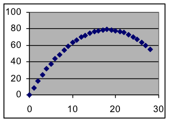
There are several ways to write a quadratic formula, all of which can make the same curves. For use in fitting data, the best kind of quadratic formula is y = a (x – h) 2 + v, where the parameters h and v are the x and y coordinates of the vertex of the parabola (that is, its highest or lowest point), and a is a “shape” parameter that determines how sharply (and in which direction) the parabola bends.

The quadratic formula pattern that is most convenient for fitting models: $y=a\cdot{{(x-h)}^{2}}+v$

a is a “shape” parameter controlling how much (and in which direction) the parabola bends

h is the x coordinate of the vertex (its horizontal distance from the origin)

v is the y coordinate of the vertex (its vertical distance from the origin)

Examples: $y=3\cdot{{(x-2)}^{2}}+8$ $y=2.5\cdot{{(x-7)}^{2}}-33.4$ $y=-2\cdot{{(x+3.5)}^{2}}+37$

time	height
x	y
0	0.0
1	8.6
2	16.8
3	24.4
4	31.5
5	37.4
6	43.8
7	48.9
8	54.4
9	58.9
10	63.3
11	66.5
12	69.7
13	72.2
14	74.5
15	76.2
16	77.8
17	78.1
18	79.0
19	78.5
20	78.0
21	76.9
22	75.6
23	73.0
24	70.3
25	67.3
26	63.7
27	60.0
28	55.0

Examples of graphs of various quadratic formulas
$graph1$	$graph2$	$graph3$	$graph4$
$y=3\cdot{{(x-2)}^{2}}+8$	$y=-1.2\cdot{{(x-2.5)}^{2}}-50$	$y=18\cdot{{(x+3)}^{2}}-158$	$y=3\cdot{{(x+7)}^{2}}-300$

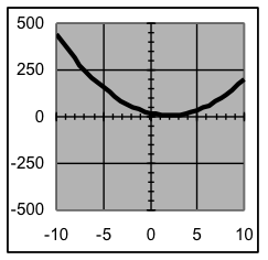
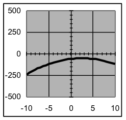
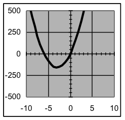
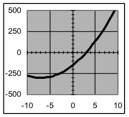
Example 5: For each of the formulas above, state the location of the vertex of the parabola formed.

Solution: Since the vertex is at (h,v) when a formula is expressed in the form, the coordinates for the vertices are: (2, 8) (2.5, −50) (−3, −158) (−7, −300)

Note that the sign of the x vertex coordinate is the opposite of the sign that the same number has in the formula, since the h value is subtracted when forming the formula.

Quadratic models are somewhat more complicated than linear ones, as is indicated by the fact that a quadratic model has three parameters instead of two. But there is really very little difference in the fitting process from what is done for straight lines: [1] put the data in the appropriate worksheet, [2] spread the C3:E3 formulas down beside the data, [3] make a graph and adjust the vertex (instead of the intercept) and the shape (instead of the slope) until the model and the data match, and [5] write down the formula or use it to predict any values you have been asked for.

Mathematics for Modeling. Authored by: Mary Parker and Hunter Ellinger. License: CC BY: Attribution

Search

Text Color

Text Size

Margin Size

Font Type