24.11: E1.10- Section 6 Part 2

Last updated
Save as PDF

Page ID: 51742

$ \newcommand{\vecs}[1]{\overset { \scriptstyle \rightharpoonup} {\mathbf{#1}} } $

$ \newcommand{\vecd}[1]{\overset{-\!-\!\rightharpoonup}{\vphantom{a}\smash {#1}}} $

$ \newcommand{\id}{\mathrm{id}}$ $ \newcommand{\Span}{\mathrm{span}}$

( \newcommand{\kernel}{\mathrm{null}\,}\) $ \newcommand{\range}{\mathrm{range}\,}$

$ \newcommand{\RealPart}{\mathrm{Re}}$ $ \newcommand{\ImaginaryPart}{\mathrm{Im}}$

$ \newcommand{\Argument}{\mathrm{Arg}}$ $ \newcommand{\norm}[1]{\| #1 \|}$

$ \newcommand{\inner}[2]{\langle #1, #2 \rangle}$

$ \newcommand{\Span}{\mathrm{span}}$

$ \newcommand{\id}{\mathrm{id}}$

$ \newcommand{\Span}{\mathrm{span}}$

$ \newcommand{\kernel}{\mathrm{null}\,}$

$ \newcommand{\range}{\mathrm{range}\,}$

$ \newcommand{\RealPart}{\mathrm{Re}}$

$ \newcommand{\ImaginaryPart}{\mathrm{Im}}$

$ \newcommand{\Argument}{\mathrm{Arg}}$

$ \newcommand{\norm}[1]{\| #1 \|}$

$ \newcommand{\inner}[2]{\langle #1, #2 \rangle}$

$ \newcommand{\Span}{\mathrm{span}}$ $ \newcommand{\AA}{\unicode[.8,0]{x212B}}$

$ \newcommand{\vectorA}[1]{\vec{#1}} % arrow$

$ \newcommand{\vectorAt}[1]{\vec{\text{#1}}} % arrow$

$ \newcommand{\vectorB}[1]{\overset { \scriptstyle \rightharpoonup} {\mathbf{#1}} } $

$ \newcommand{\vectorC}[1]{\textbf{#1}} $

$ \newcommand{\vectorD}[1]{\overrightarrow{#1}} $

$ \newcommand{\vectorDt}[1]{\overrightarrow{\text{#1}}} $

$ \newcommand{\vectE}[1]{\overset{-\!-\!\rightharpoonup}{\vphantom{a}\smash{\mathbf {#1}}}} $

$ \newcommand{\vecs}[1]{\overset { \scriptstyle \rightharpoonup} {\mathbf{#1}} } $

$ \newcommand{\vecd}[1]{\overset{-\!-\!\rightharpoonup}{\vphantom{a}\smash {#1}}} $

$\newcommand{\avec}{\mathbf a}$ $\newcommand{\bvec}{\mathbf b}$ $\newcommand{\cvec}{\mathbf c}$ $\newcommand{\dvec}{\mathbf d}$ $\newcommand{\dtil}{\widetilde{\mathbf d}}$ $\newcommand{\evec}{\mathbf e}$ $\newcommand{\fvec}{\mathbf f}$ $\newcommand{\nvec}{\mathbf n}$ $\newcommand{\pvec}{\mathbf p}$ $\newcommand{\qvec}{\mathbf q}$ $\newcommand{\svec}{\mathbf s}$ $\newcommand{\tvec}{\mathbf t}$ $\newcommand{\uvec}{\mathbf u}$ $\newcommand{\vvec}{\mathbf v}$ $\newcommand{\wvec}{\mathbf w}$ $\newcommand{\xvec}{\mathbf x}$ $\newcommand{\yvec}{\mathbf y}$ $\newcommand{\zvec}{\mathbf z}$ $\newcommand{\rvec}{\mathbf r}$ $\newcommand{\mvec}{\mathbf m}$ $\newcommand{\zerovec}{\mathbf 0}$ $\newcommand{\onevec}{\mathbf 1}$ $\newcommand{\real}{\mathbb R}$ $\newcommand{\twovec}[2]{\left[\begin{array}{r}#1 \\ #2 \end{array}\right]}$ $\newcommand{\ctwovec}[2]{\left[\begin{array}{c}#1 \\ #2 \end{array}\right]}$ $\newcommand{\threevec}[3]{\left[\begin{array}{r}#1 \\ #2 \\ #3 \end{array}\right]}$ $\newcommand{\cthreevec}[3]{\left[\begin{array}{c}#1 \\ #2 \\ #3 \end{array}\right]}$ $\newcommand{\fourvec}[4]{\left[\begin{array}{r}#1 \\ #2 \\ #3 \\ #4 \end{array}\right]}$ $\newcommand{\cfourvec}[4]{\left[\begin{array}{c}#1 \\ #2 \\ #3 \\ #4 \end{array}\right]}$ $\newcommand{\fivevec}[5]{\left[\begin{array}{r}#1 \\ #2 \\ #3 \\ #4 \\ #5 \\ \end{array}\right]}$ $\newcommand{\cfivevec}[5]{\left[\begin{array}{c}#1 \\ #2 \\ #3 \\ #4 \\ #5 \\ \end{array}\right]}$ $\newcommand{\mattwo}[4]{\left[\begin{array}{rr}#1 \amp #2 \\ #3 \amp #4 \\ \end{array}\right]}$ $\newcommand{\laspan}[1]{\text{Span}\{#1\}}$ $\newcommand{\bcal}{\cal B}$ $\newcommand{\ccal}{\cal C}$ $\newcommand{\scal}{\cal S}$ $\newcommand{\wcal}{\cal W}$ $\newcommand{\ecal}{\cal E}$ $\newcommand{\coords}[2]{\left\{#1\right\}_{#2}}$ $\newcommand{\gray}[1]{\color{gray}{#1}}$ $\newcommand{\lgray}[1]{\color{lightgray}{#1}}$ $\newcommand{\rank}{\operatorname{rank}}$ $\newcommand{\row}{\text{Row}}$ $\newcommand{\col}{\text{Col}}$ $\renewcommand{\row}{\text{Row}}$ $\newcommand{\nul}{\text{Nul}}$ $\newcommand{\var}{\text{Var}}$ $\newcommand{\corr}{\text{corr}}$ $\newcommand{\len}[1]{\left|#1\right|}$ $\newcommand{\bbar}{\overline{\bvec}}$ $\newcommand{\bhat}{\widehat{\bvec}}$ $\newcommand{\bperp}{\bvec^\perp}$ $\newcommand{\xhat}{\widehat{\xvec}}$ $\newcommand{\vhat}{\widehat{\vvec}}$ $\newcommand{\uhat}{\widehat{\uvec}}$ $\newcommand{\what}{\widehat{\wvec}}$ $\newcommand{\Sighat}{\widehat{\Sigma}}$ $\newcommand{\lt}{<}$ $\newcommand{\gt}{>}$ $\newcommand{\amp}{&}$ $\definecolor{fillinmathshade}{gray}{0.9}$

Start exploring. How does changing h change the graph?

Start by changing h to -2.

That makes the spreadsheet look like the illustration below.

	A	B	C	D	E	F	G	H
1	x	y
2	-6	36					2	a
3	-5	22					-2	h
4	-4	12					4	k
5	-3	6
6	-2	4
7	-1	6
8	0	12
9	1	22
10	2	36
11	3	54
12	4	76
13	5	102
14	6	132
15
16

$122.png$

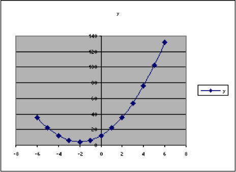
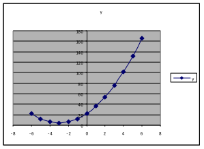
Now we can notice that, when $h=3$ , the lowest point on the graph is at $x=3$ , and when $h=-2$ , then the lowest point on the graph is at $x=-2$ .

This suggests that maybe the value that is subtracted from x in the original formula is the one that determines where the lowest y-value is – that is, where the lowest point on the graph is.

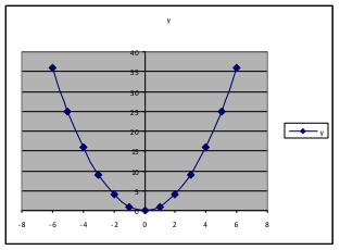
Try $h=0$ , $h=4$ , and $h=-3$ .

$h=0$

(leaving $a=2$ and $k=4$ )

$h=4$

(leaving $a=2$ and $k=4$ )

$h=-3$

(leaving $a=2$ and $k=4$ )

$211.png$

$35.png$

$43.png$

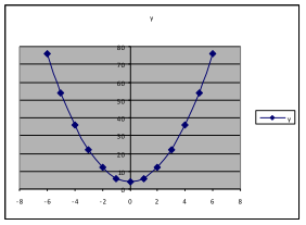Do these results support the conjecture we made in the previous sentence? Answer: Yes.

Example 21. Using the same formula and spreadsheet as in Example 18, use the values $a=1$ , $h=0$ , and explore the effect of changing k.

$k=4$

(leaving $a=1$ and $h=0$ )

$k=0$

(leaving $a=1$ and $h=0$ )

$k=-7$

(leaving $a=1$ and $h=0$ )

$53.png$

$36.png$

$44.png$

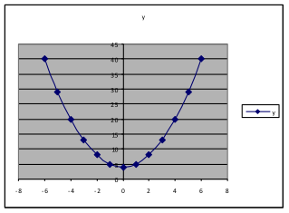We find that changing k alone changes how far up or down the lowest point on the graph is. It appears that the y-value of that lowest point is k.

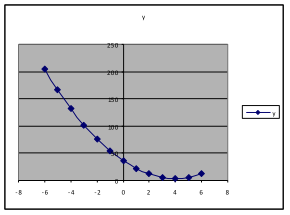
Example 22. Using the same formula and spreadsheet as in Example 17, use $h=0$ and $k=0$ , and explore the effect of changing a.

$a=1$

(with $h=0$ and $k=0$ )

$a=3$

(with $h=0$ and $k=0$ )

$a=-3$

(with $h=0$ and $k=0$ )

$82.png$

$91.png$

$101.png$

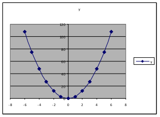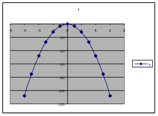We find that changing a from a positive to a negative number makes the graph change from opening upward to opening downward. Making a larger (from 1 to 3) changes how large the y-values are, so that the y-values for $a=3$ are three times as large as those when $a=1$ .

Mathematics for Modeling. Authored by: Mary Parker and Hunter Ellinger. License: CC BY: Attribution

Search

Text Color

Text Size

Margin Size

Font Type

	A	B	C	D	E	F	G	H
1	x	y
2	-6	36					2	a
3	-5	22					-2	h
4	-4	12					4	k
5	-3	6
6	-2	4
7	-1	6
8	0	12
9	1	22
10	2	36
11	3	54
12	4	76
13	5	102
14	6	132
15
16

	A	B	C	D	E	F	G	H
1	x	y
2	-6	36					2	a
3	-5	22					-2	h
4	-4	12					4	k
5	-3	6
6	-2	4
7	-1	6
8	0	12
9	1	22
10	2	36
11	3	54
12	4	76
13	5	102
14	6	132
15
16

	A	B	C	D	E	F	G	H
1	x	y
2	-6	36					2	a
3	-5	22					-2	h
4	-4	12					4	k
5	-3	6
6	-2	4
7	-1	6
8	0	12
9	1	22
10	2	36
11	3	54
12	4	76
13	5	102
14	6	132
15
16