8.6: Hypothesis Test of a Single Population Mean with Examples

Last updated
Save as PDF

Page ID: 130297

Zoya Kravets
Mission College

$ \newcommand{\vecs}[1]{\overset { \scriptstyle \rightharpoonup} {\mathbf{#1}} } $

$ \newcommand{\vecd}[1]{\overset{-\!-\!\rightharpoonup}{\vphantom{a}\smash {#1}}} $

$ \newcommand{\id}{\mathrm{id}}$ $ \newcommand{\Span}{\mathrm{span}}$

( \newcommand{\kernel}{\mathrm{null}\,}\) $ \newcommand{\range}{\mathrm{range}\,}$

$ \newcommand{\RealPart}{\mathrm{Re}}$ $ \newcommand{\ImaginaryPart}{\mathrm{Im}}$

$ \newcommand{\Argument}{\mathrm{Arg}}$ $ \newcommand{\norm}[1]{\| #1 \|}$

$ \newcommand{\inner}[2]{\langle #1, #2 \rangle}$

$ \newcommand{\Span}{\mathrm{span}}$

$ \newcommand{\id}{\mathrm{id}}$

$ \newcommand{\Span}{\mathrm{span}}$

$ \newcommand{\kernel}{\mathrm{null}\,}$

$ \newcommand{\range}{\mathrm{range}\,}$

$ \newcommand{\RealPart}{\mathrm{Re}}$

$ \newcommand{\ImaginaryPart}{\mathrm{Im}}$

$ \newcommand{\Argument}{\mathrm{Arg}}$

$ \newcommand{\norm}[1]{\| #1 \|}$

$ \newcommand{\inner}[2]{\langle #1, #2 \rangle}$

$ \newcommand{\Span}{\mathrm{span}}$ $ \newcommand{\AA}{\unicode[.8,0]{x212B}}$

$ \newcommand{\vectorA}[1]{\vec{#1}} % arrow$

$ \newcommand{\vectorAt}[1]{\vec{\text{#1}}} % arrow$

$ \newcommand{\vectorB}[1]{\overset { \scriptstyle \rightharpoonup} {\mathbf{#1}} } $

$ \newcommand{\vectorC}[1]{\textbf{#1}} $

$ \newcommand{\vectorD}[1]{\overrightarrow{#1}} $

$ \newcommand{\vectorDt}[1]{\overrightarrow{\text{#1}}} $

$ \newcommand{\vectE}[1]{\overset{-\!-\!\rightharpoonup}{\vphantom{a}\smash{\mathbf {#1}}}} $

$ \newcommand{\vecs}[1]{\overset { \scriptstyle \rightharpoonup} {\mathbf{#1}} } $

$ \newcommand{\vecd}[1]{\overset{-\!-\!\rightharpoonup}{\vphantom{a}\smash {#1}}} $

$\newcommand{\avec}{\mathbf a}$ $\newcommand{\bvec}{\mathbf b}$ $\newcommand{\cvec}{\mathbf c}$ $\newcommand{\dvec}{\mathbf d}$ $\newcommand{\dtil}{\widetilde{\mathbf d}}$ $\newcommand{\evec}{\mathbf e}$ $\newcommand{\fvec}{\mathbf f}$ $\newcommand{\nvec}{\mathbf n}$ $\newcommand{\pvec}{\mathbf p}$ $\newcommand{\qvec}{\mathbf q}$ $\newcommand{\svec}{\mathbf s}$ $\newcommand{\tvec}{\mathbf t}$ $\newcommand{\uvec}{\mathbf u}$ $\newcommand{\vvec}{\mathbf v}$ $\newcommand{\wvec}{\mathbf w}$ $\newcommand{\xvec}{\mathbf x}$ $\newcommand{\yvec}{\mathbf y}$ $\newcommand{\zvec}{\mathbf z}$ $\newcommand{\rvec}{\mathbf r}$ $\newcommand{\mvec}{\mathbf m}$ $\newcommand{\zerovec}{\mathbf 0}$ $\newcommand{\onevec}{\mathbf 1}$ $\newcommand{\real}{\mathbb R}$ $\newcommand{\twovec}[2]{\left[\begin{array}{r}#1 \\ #2 \end{array}\right]}$ $\newcommand{\ctwovec}[2]{\left[\begin{array}{c}#1 \\ #2 \end{array}\right]}$ $\newcommand{\threevec}[3]{\left[\begin{array}{r}#1 \\ #2 \\ #3 \end{array}\right]}$ $\newcommand{\cthreevec}[3]{\left[\begin{array}{c}#1 \\ #2 \\ #3 \end{array}\right]}$ $\newcommand{\fourvec}[4]{\left[\begin{array}{r}#1 \\ #2 \\ #3 \\ #4 \end{array}\right]}$ $\newcommand{\cfourvec}[4]{\left[\begin{array}{c}#1 \\ #2 \\ #3 \\ #4 \end{array}\right]}$ $\newcommand{\fivevec}[5]{\left[\begin{array}{r}#1 \\ #2 \\ #3 \\ #4 \\ #5 \\ \end{array}\right]}$ $\newcommand{\cfivevec}[5]{\left[\begin{array}{c}#1 \\ #2 \\ #3 \\ #4 \\ #5 \\ \end{array}\right]}$ $\newcommand{\mattwo}[4]{\left[\begin{array}{rr}#1 \amp #2 \\ #3 \amp #4 \\ \end{array}\right]}$ $\newcommand{\laspan}[1]{\text{Span}\{#1\}}$ $\newcommand{\bcal}{\cal B}$ $\newcommand{\ccal}{\cal C}$ $\newcommand{\scal}{\cal S}$ $\newcommand{\wcal}{\cal W}$ $\newcommand{\ecal}{\cal E}$ $\newcommand{\coords}[2]{\left\{#1\right\}_{#2}}$ $\newcommand{\gray}[1]{\color{gray}{#1}}$ $\newcommand{\lgray}[1]{\color{lightgray}{#1}}$ $\newcommand{\rank}{\operatorname{rank}}$ $\newcommand{\row}{\text{Row}}$ $\newcommand{\col}{\text{Col}}$ $\renewcommand{\row}{\text{Row}}$ $\newcommand{\nul}{\text{Nul}}$ $\newcommand{\var}{\text{Var}}$ $\newcommand{\corr}{\text{corr}}$ $\newcommand{\len}[1]{\left|#1\right|}$ $\newcommand{\bbar}{\overline{\bvec}}$ $\newcommand{\bhat}{\widehat{\bvec}}$ $\newcommand{\bperp}{\bvec^\perp}$ $\newcommand{\xhat}{\widehat{\xvec}}$ $\newcommand{\vhat}{\widehat{\vvec}}$ $\newcommand{\uhat}{\widehat{\uvec}}$ $\newcommand{\what}{\widehat{\wvec}}$ $\newcommand{\Sighat}{\widehat{\Sigma}}$ $\newcommand{\lt}{<}$ $\newcommand{\gt}{>}$ $\newcommand{\amp}{&}$ $\definecolor{fillinmathshade}{gray}{0.9}$

Steps for performing Hypothesis Test of a Single Population Mean

Step 1: State your hypotheses about the population mean.
Step 2: Summarize the data. State a significance level. State and check conditions required for the procedure

Find or identify the sample size, n, the sample mean, $\bar{x}$ and the sample standard deviation, s.

The sampling distribution for the one-mean test statistic is, approximately, T- distribution if the following conditions are met

Sample is random with independent observations.
Sample is large. The population must be Normal or the sample size must be at least 30.

Step 3: Perform the procedure based on the assumption that $H_{0}$ is true

Find the Estimated Standard Error: $SE=\frac{s}{\sqrt{n}}$.
Compute the observed value of the test statistic: $T_{obs}=\frac{\bar{x}-\mu_{0}}{SE}$.
Check the type of the test (right-, left-, or two-tailed)
Find the p-value in order to measure your level of surprise.

Step 4: Make a decision about $H_{0}$ and $H_{a}$

Do you reject or not reject your null hypothesis?

Step 5: Make a conclusion

What does this mean in the context of the data?

The following examples illustrate a left-, right-, and two-tailed test.

Example $\PageIndex{1}$

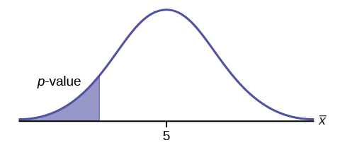
$H_{0}: \mu = 5, H_{a}: \mu < 5$

Test of a single population mean. $H_{a}$ tells you the test is left-tailed. The picture of the $p$-value is as follows:

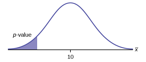
Normal distribution curve of a single population mean with a value of 5 on the x-axis and the p-value points to the area on the left tail of the curve. — Figure $\PageIndex{1}$

Exercise $\PageIndex{1}$

$H_{0}: \mu = 10, H_{a}: \mu < 10$

Assume the $p$-value is 0.0935. What type of test is this? Draw the picture of the $p$-value.

Answer

left-tailed test

Example $\PageIndex{2}$

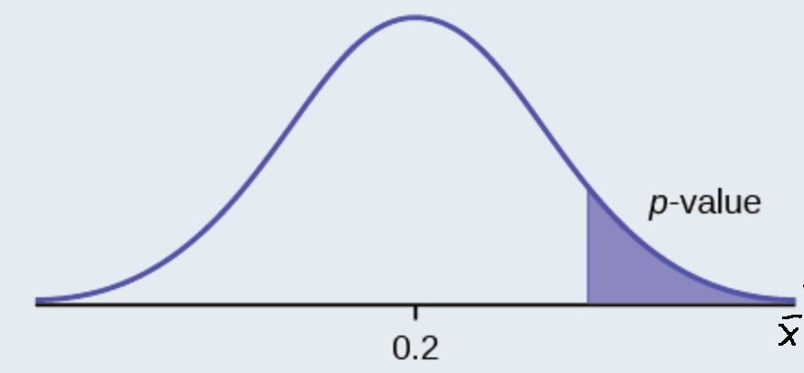
$H_{0}: \mu \leq 0.2, H_{a}: \mu > 0.2$

This is a test of a single population proportion. $H_{a}$ tells you the test is right-tailed. The picture of the p-value is as follows:

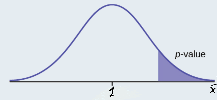
Normal distribution curve of a single population proportion with the value of 0.2 on the x-axis. The p-value points to the area on the right tail of the curve. — Figure $\PageIndex{3}$

Exercise $\PageIndex{2}$

$H_{0}: \mu \leq 1, H_{a}: \mu > 1$

Assume the $p$-value is 0.1243. What type of test is this? Draw the picture of the $p$-value.

Answer

right-tailed test

Example $\PageIndex{3}$

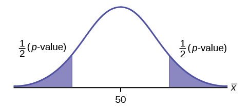
$H_{0}: \mu = 50, H_{a}: \mu \neq 50$

This is a test of a single population mean. $H_{a}$ tells you the test is two-tailed. The picture of the $p$-value is as follows.

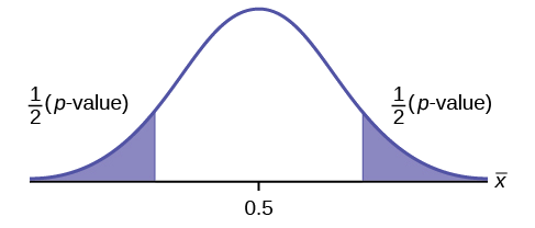
Normal distribution curve of a single population mean with a value of 50 on the x-axis. The p-value formulas, 1/2(p-value), for a two-tailed test is shown for the areas on the left and right tails of the curve. — Figure $\PageIndex{5}$

Exercise $\PageIndex{3}$

$H_{0}: \mu = 0.5, H_{a}: \mu \neq 0.5$

Assume the p-value is 0.2564. What type of test is this? Draw the picture of the $p$-value.

Answer

two-tailed test

Full Hypothesis Test Examples

Example $\PageIndex{4}$

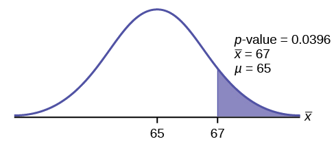
Statistics students believe that the mean score on the first statistics test is 65. A statistics instructor thinks the mean score is higher than 65. He samples ten statistics students and obtains the scores 65 65 70 67 66 63 63 68 72 71. He performs a hypothesis test using a 5% level of significance. The data are assumed to be from a normal distribution.

Answer

Set up the hypothesis test:

A 5% level of significance means that $\alpha = 0.05$. This is a test of a single population mean.

$H_{0}: \mu = 65 H_{a}: \mu > 65$

Since the instructor thinks the average score is higher, use a "$>$". The "$>$" means the test is right-tailed.

Determine the distribution needed:

Random variable: $\bar{X} =$ average score on the first statistics test.

Distribution for the test: If you read the problem carefully, you will notice that there is no population standard deviation given. You are only given $n = 10$ sample data values. Notice also that the data come from a normal distribution. This means that the distribution for the test is a student's $t$.

Use $t_{df}$. Therefore, the distribution for the test is $t_{9}$ where $n = 10$ and $df = 10 - 1 = 9$.

The sample mean and sample standard deviation are calculated as 67 and 3.1972 from the data.

Calculate the $p$-value using the Student's $t$-distribution:

\[t_{obs} = \dfrac{\bar{x}-\mu_{\bar{x}}}{\left(\dfrac{s}{\sqrt{n}}\right)}=\dfrac{67-65}{\left(\dfrac{3.1972}{\sqrt{10}}\right)}\]

Use the T-table or Excel's t_dist() function to find p-value:

$p\text{-value} = P(\bar{x} > 67) =P(T >1.9782 )= 1-0.9604=0.0396$

Interpretation of the p-value: If the null hypothesis is true, then there is a 0.0396 probability (3.96%) that the sample mean is 65 or more.

Normal distribution curve of average scores on the first statistic tests with 65 and 67 values on the x-axis. A vertical upward line extends from 67 to the curve. The p-value points to the area to the right of 67. — Figure $\PageIndex{11}$

Compare $\alpha$ and the $p-\text{value}$:

Since $α = 0.05$ and $p\text{-value} = 0.0396$. $\alpha > p\text{-value}$.

Make a decision: Since $\alpha > p\text{-value}$, reject $H_{0}$.

This means you reject $\mu = 65$. In other words, you believe the average test score is more than 65.

Conclusion: At a 5% level of significance, the sample data show sufficient evidence that the mean (average) test score is more than 65, just as the math instructor thinks.

The $p\text{-value}$ can easily be calculated.

Put the data into a list. Press STAT and arrow over to TESTS. Press 2:T-Test. Arrow over to Data and press ENTER. Arrow down and enter 65 for $\mu_{0}$, the name of the list where you put the data, and 1 for Freq:. Arrow down to $\mu$: and arrow over to $> \mu_{0}$. Press ENTER. Arrow down to Calculate and pressENTER. The calculator not only calculates the $p\text{-value}$ (p = 0.0396) but it also calculates the test statistic (t-score) for the sample mean, the sample mean, and the sample standard deviation. $\mu > 65$ is the alternative hypothesis. Do this set of instructions again except arrow to Draw (instead of Calculate). Press ENTER. A shaded graph appears with $t = 1.9781$ (test statistic) and $p = 0.0396$ ($p\text{-value}$). Make sure when you use Draw that no other equations are highlighted in $Y =$ and the plots are turned off.

Exercise $\PageIndex{4}$

It is believed that a stock price for a particular company will grow at a rate of $5 per week with a standard deviation of $1. An investor believes the stock won’t grow as quickly. The changes in stock price is recorded for ten weeks and are as follows: $4, $3, $2, $3, $1, $7, $2, $1, $1, $2. Perform a hypothesis test using a 5% level of significance. State the null and alternative hypotheses, find the p-value, state your conclusion, and identify the Type I and Type II errors.

Answer

$H_{0}: \mu = 5$
$H_{a}: \mu < 5$
$p = 0.0082$

Because $p < \alpha$, we reject the null hypothesis. There is sufficient evidence to suggest that the stock price of the company grows at a rate less than $5 a week.

Type I Error: To conclude that the stock price is growing slower than $5 a week when, in fact, the stock price is growing at $5 a week (reject the null hypothesis when the null hypothesis is true).
Type II Error: To conclude that the stock price is growing at a rate of $5 a week when, in fact, the stock price is growing slower than $5 a week (do not reject the null hypothesis when the null hypothesis is false).

Example $\PageIndex{5}$

The National Institute of Standards and Technology provides exact data on conductivity properties of materials. Following are conductivity measurements for 11 randomly selected pieces of a particular type of glass.

1.11; 1.07; 1.11; 1.07; 1.12; 1.08; .98; .98 1.02; .95; .95

Is there convincing evidence that the average conductivity of this type of glass is greater than one? Use a significance level of 0.05. Assume the population is normal.

Answer

Let’s follow a four-step process to answer this statistical question.

State the Question: We need to determine if, at a 0.05 significance level, the average conductivity of the selected glass is greater than one. Our hypotheses will be
1. $H_{0}: \mu \leq 1$
2. $H_{a}: \mu > 1$
Plan: We are testing a sample mean without a known population standard deviation. Therefore, we need to use a Student's-t distribution. Assume the underlying population is normal.
Do the calculations: $p\text{-value} ( = 0.036)$

4. State the Conclusions: Since the $p\text{-value} (= 0.036)$ is less than our alpha value, we will reject the null hypothesis. It is reasonable to state that the data supports the claim that the average conductivity level is greater than one.

Review

The hypothesis test itself has an established process. This can be summarized as follows:

Determine $H_{0}$ and $H_{a}$. Remember, they are contradictory.
Determine the random variable.
Determine the distribution for the test.
Draw a graph, calculate the test statistic, and use the test statistic to calculate the $p\text{-value}$. (A t-score is an example of test statistics.)
Compare the preconceived α with the p-value, make a decision (reject or do not reject H₀), and write a clear conclusion using English sentences.

Notice that in performing the hypothesis test, you use $\alpha$ and not $\beta$. $\beta$ is needed to help determine the sample size of the data that is used in calculating the $p\text{-value}$. Remember that the quantity $1 – \beta$ is called the Power of the Test. A high power is desirable. If the power is too low, statisticians typically increase the sample size while keeping α the same.If the power is low, the null hypothesis might not be rejected when it should be.

References

Data from Amit Schitai. Director of Instructional Technology and Distance Learning. LBCC.
Data from Bloomberg Businessweek. Available online at www.businessweek.com/news/2011- 09-15/nyc-smoking-rate-falls-to-record-low-of-14-bloomberg-says.html.
Data from energy.gov. Available online at http://energy.gov (accessed June 27. 2013).
Data from Gallup®. Available online at www.gallup.com (accessed June 27, 2013).
Data from Growing by Degrees by Allen and Seaman.
Data from La Leche League International. Available online at www.lalecheleague.org/Law/BAFeb01.html.
Data from the American Automobile Association. Available online at www.aaa.com (accessed June 27, 2013).
Data from the American Library Association. Available online at www.ala.org (accessed June 27, 2013).
Data from the Bureau of Labor Statistics. Available online at http://www.bls.gov/oes/current/oes291111.htm.
Data from the Centers for Disease Control and Prevention. Available online at www.cdc.gov (accessed June 27, 2013)
Data from the U.S. Census Bureau, available online at quickfacts.census.gov/qfd/states/00000.html (accessed June 27, 2013).
Data from the United States Census Bureau. Available online at www.census.gov/hhes/socdemo/language/.
Data from Toastmasters International. Available online at http://toastmasters.org/artisan/deta...eID=429&Page=1.
Data from Weather Underground. Available online at www.wunderground.com (accessed June 27, 2013).
Federal Bureau of Investigations. “Uniform Crime Reports and Index of Crime in Daviess in the State of Kentucky enforced by Daviess County from 1985 to 2005.” Available online at http://www.disastercenter.com/kentucky/crime/3868.htm (accessed June 27, 2013).
“Foothill-De Anza Community College District.” De Anza College, Winter 2006. Available online at research.fhda.edu/factbook/DA...t_da_2006w.pdf.
Johansen, C., J. Boice, Jr., J. McLaughlin, J. Olsen. “Cellular Telephones and Cancer—a Nationwide Cohort Study in Denmark.” Institute of Cancer Epidemiology and the Danish Cancer Society, 93(3):203-7. Available online at http://www.ncbi.nlm.nih.gov/pubmed/11158188 (accessed June 27, 2013).
Rape, Abuse & Incest National Network. “How often does sexual assault occur?” RAINN, 2009. Available online at www.rainn.org/get-information...sexual-assault (accessed June 27, 2013).

Glossary

Central Limit Theorem: Given a random variable (RV) with known mean $\mu$ and known standard deviation $\sigma$. We are sampling with size $n$ and we are interested in two new RVs - the sample mean, $\bar{X}$, and the sample sum, $\sum X$. If the size $n$ of the sample is sufficiently large, then $\bar{X} - N\left(\mu, \frac{\sigma}{\sqrt{n}}\right)$ and $\sum X - N \left(n\mu, \sqrt{n}\sigma\right)$. If the size n of the sample is sufficiently large, then the distribution of the sample means and the distribution of the sample sums will approximate a normal distribution regardless of the shape of the population. The mean of the sample means will equal the population mean and the mean of the sample sums will equal $n$ times the population mean. The standard deviation of the distribution of the sample means, $\frac{\sigma}{\sqrt{n}}$, is called the standard error of the mean.

Search

Text Color

Text Size

Margin Size

Font Type

Example \(\PageIndex{1}\)

Exercise \(\PageIndex{1}\)

Example \(\PageIndex{2}\)

Exercise \(\PageIndex{2}\)

Example \(\PageIndex{3}\)

Exercise \(\PageIndex{3}\)

Example \(\PageIndex{4}\)

Exercise \(\PageIndex{4}\)

Example \(\PageIndex{5}\)