2.3E: Exercises for Section 2.3

Last updated
Save as PDF

Page ID: 112045

$ \newcommand{\vecs}[1]{\overset { \scriptstyle \rightharpoonup} {\mathbf{#1}} } $

$ \newcommand{\vecd}[1]{\overset{-\!-\!\rightharpoonup}{\vphantom{a}\smash {#1}}} $

$ \newcommand{\id}{\mathrm{id}}$ $ \newcommand{\Span}{\mathrm{span}}$

( \newcommand{\kernel}{\mathrm{null}\,}\) $ \newcommand{\range}{\mathrm{range}\,}$

$ \newcommand{\RealPart}{\mathrm{Re}}$ $ \newcommand{\ImaginaryPart}{\mathrm{Im}}$

$ \newcommand{\Argument}{\mathrm{Arg}}$ $ \newcommand{\norm}[1]{\| #1 \|}$

$ \newcommand{\inner}[2]{\langle #1, #2 \rangle}$

$ \newcommand{\Span}{\mathrm{span}}$

$ \newcommand{\id}{\mathrm{id}}$

$ \newcommand{\Span}{\mathrm{span}}$

$ \newcommand{\kernel}{\mathrm{null}\,}$

$ \newcommand{\range}{\mathrm{range}\,}$

$ \newcommand{\RealPart}{\mathrm{Re}}$

$ \newcommand{\ImaginaryPart}{\mathrm{Im}}$

$ \newcommand{\Argument}{\mathrm{Arg}}$

$ \newcommand{\norm}[1]{\| #1 \|}$

$ \newcommand{\inner}[2]{\langle #1, #2 \rangle}$

$ \newcommand{\Span}{\mathrm{span}}$ $ \newcommand{\AA}{\unicode[.8,0]{x212B}}$

$ \newcommand{\vectorA}[1]{\vec{#1}} % arrow$

$ \newcommand{\vectorAt}[1]{\vec{\text{#1}}} % arrow$

$ \newcommand{\vectorB}[1]{\overset { \scriptstyle \rightharpoonup} {\mathbf{#1}} } $

$ \newcommand{\vectorC}[1]{\textbf{#1}} $

$ \newcommand{\vectorD}[1]{\overrightarrow{#1}} $

$ \newcommand{\vectorDt}[1]{\overrightarrow{\text{#1}}} $

$ \newcommand{\vectE}[1]{\overset{-\!-\!\rightharpoonup}{\vphantom{a}\smash{\mathbf {#1}}}} $

$ \newcommand{\vecs}[1]{\overset { \scriptstyle \rightharpoonup} {\mathbf{#1}} } $

$ \newcommand{\vecd}[1]{\overset{-\!-\!\rightharpoonup}{\vphantom{a}\smash {#1}}} $

$\newcommand{\avec}{\mathbf a}$ $\newcommand{\bvec}{\mathbf b}$ $\newcommand{\cvec}{\mathbf c}$ $\newcommand{\dvec}{\mathbf d}$ $\newcommand{\dtil}{\widetilde{\mathbf d}}$ $\newcommand{\evec}{\mathbf e}$ $\newcommand{\fvec}{\mathbf f}$ $\newcommand{\nvec}{\mathbf n}$ $\newcommand{\pvec}{\mathbf p}$ $\newcommand{\qvec}{\mathbf q}$ $\newcommand{\svec}{\mathbf s}$ $\newcommand{\tvec}{\mathbf t}$ $\newcommand{\uvec}{\mathbf u}$ $\newcommand{\vvec}{\mathbf v}$ $\newcommand{\wvec}{\mathbf w}$ $\newcommand{\xvec}{\mathbf x}$ $\newcommand{\yvec}{\mathbf y}$ $\newcommand{\zvec}{\mathbf z}$ $\newcommand{\rvec}{\mathbf r}$ $\newcommand{\mvec}{\mathbf m}$ $\newcommand{\zerovec}{\mathbf 0}$ $\newcommand{\onevec}{\mathbf 1}$ $\newcommand{\real}{\mathbb R}$ $\newcommand{\twovec}[2]{\left[\begin{array}{r}#1 \\ #2 \end{array}\right]}$ $\newcommand{\ctwovec}[2]{\left[\begin{array}{c}#1 \\ #2 \end{array}\right]}$ $\newcommand{\threevec}[3]{\left[\begin{array}{r}#1 \\ #2 \\ #3 \end{array}\right]}$ $\newcommand{\cthreevec}[3]{\left[\begin{array}{c}#1 \\ #2 \\ #3 \end{array}\right]}$ $\newcommand{\fourvec}[4]{\left[\begin{array}{r}#1 \\ #2 \\ #3 \\ #4 \end{array}\right]}$ $\newcommand{\cfourvec}[4]{\left[\begin{array}{c}#1 \\ #2 \\ #3 \\ #4 \end{array}\right]}$ $\newcommand{\fivevec}[5]{\left[\begin{array}{r}#1 \\ #2 \\ #3 \\ #4 \\ #5 \\ \end{array}\right]}$ $\newcommand{\cfivevec}[5]{\left[\begin{array}{c}#1 \\ #2 \\ #3 \\ #4 \\ #5 \\ \end{array}\right]}$ $\newcommand{\mattwo}[4]{\left[\begin{array}{rr}#1 \amp #2 \\ #3 \amp #4 \\ \end{array}\right]}$ $\newcommand{\laspan}[1]{\text{Span}\{#1\}}$ $\newcommand{\bcal}{\cal B}$ $\newcommand{\ccal}{\cal C}$ $\newcommand{\scal}{\cal S}$ $\newcommand{\wcal}{\cal W}$ $\newcommand{\ecal}{\cal E}$ $\newcommand{\coords}[2]{\left\{#1\right\}_{#2}}$ $\newcommand{\gray}[1]{\color{gray}{#1}}$ $\newcommand{\lgray}[1]{\color{lightgray}{#1}}$ $\newcommand{\rank}{\operatorname{rank}}$ $\newcommand{\row}{\text{Row}}$ $\newcommand{\col}{\text{Col}}$ $\renewcommand{\row}{\text{Row}}$ $\newcommand{\nul}{\text{Nul}}$ $\newcommand{\var}{\text{Var}}$ $\newcommand{\corr}{\text{corr}}$ $\newcommand{\len}[1]{\left|#1\right|}$ $\newcommand{\bbar}{\overline{\bvec}}$ $\newcommand{\bhat}{\widehat{\bvec}}$ $\newcommand{\bperp}{\bvec^\perp}$ $\newcommand{\xhat}{\widehat{\xvec}}$ $\newcommand{\vhat}{\widehat{\vvec}}$ $\newcommand{\uhat}{\widehat{\uvec}}$ $\newcommand{\what}{\widehat{\wvec}}$ $\newcommand{\Sighat}{\widehat{\Sigma}}$ $\newcommand{\lt}{<}$ $\newcommand{\gt}{>}$ $\newcommand{\amp}{&}$ $\definecolor{fillinmathshade}{gray}{0.9}$

In exercises 1 - 4, use the limit laws to evaluate each limit. Justify each step by indicating the appropriate limit law(s).

1) $\displaystyle \lim_{x→0}\,(4x^2−2x+3)$

Answer

Use constant multiple law and difference law:

$\displaystyle \lim_{x→0}\,(4x^2−2x+3)=4\lim_{x→0}x^2−2\lim_{x→0}x+\lim_{x→0}3=0 + 0 + 3=3$

2) $\displaystyle \lim_{x→1}\frac{x^3+3x^2+5}{4−7x}$

3) $\displaystyle \lim_{x→−2}\sqrt{x^2−6x+3}$

Answer: Use root law: $\displaystyle \lim_{x→−2}\sqrt{x^2−6x+3}=\sqrt{\lim_{x→−2}(x^2−6x+3)}=\sqrt{19}$

4) $\displaystyle \lim_{x→−1}(9x+1)^2$

In exercises 5 - 10, use direct substitution to evaluate the limit of each continuous function.

5) $\displaystyle \lim_{x→7}x^2$

Answer: $\displaystyle \lim_{x→7}x^2\;=\;49$

6) $\displaystyle \lim_{x→−2}(4x^2−1)$

7) $\displaystyle \lim_{x→0}\frac{1}{1+\sin x}$

Answer: $\displaystyle \lim_{x→0}\frac{1}{1+\sin x}\;=\;1$

8) $\displaystyle \lim_{x→2}e^{2x−x^2}$

9) $\displaystyle \lim_{x→1}\frac{2−7x}{x+6}$

Answer: $\displaystyle \lim_{x→1}\frac{2−7x}{x+6}\;=\;−\frac{5}{7}$

10) $\displaystyle \lim_{x→3}\ln e^{3x}$

In exercises 11 - 20, use direct substitution to show that each limit leads to the indeterminate form $0/0$. Then, evaluate the limit analytically.

11) $\displaystyle \lim_{x→4}\frac{x^2−16}{x−4}$

Answer: $\displaystyle \text{When }x = 4, \quad\frac{x^2−16}{x−4}=\frac{16−16}{4−4}=\frac{0}{0};$

then, $\displaystyle \lim_{x→4}\frac{x^2−16}{x−4}= \lim_{x→4}\frac{(x+4)(x−4)}{x−4}=\lim_{x→4}(x+4) = 4+4 =8$

12) $\displaystyle \lim_{x→2}\frac{x−2}{x^2−2x}$

13) $\displaystyle \lim_{x→6}\frac{3x−18}{2x−12}$

Answer: $\displaystyle \text{When }x = 6, \quad\frac{3x−18}{2x−12}=\frac{18−18}{12−12}=\frac{0}{0};$

then, $\displaystyle \lim_{x→6}\frac{3x−18}{2x− 12}=\lim_{x→6}\frac{3(x−6)}{2(x−6)}=\lim_{x→6}\frac{3}{2}=\frac{3}{2}$

14) $\displaystyle \lim_{h→0}\frac{(1+h)^2−1}{h}$

15) $\displaystyle \lim_{t→9}\frac{t−9}{\sqrt{t}−3}$

Answer: $\displaystyle \text{When }t = 9, \quad\frac{t−9}{\sqrt{t}−3}=\frac{9−9}{3−3}=\frac{0}{0};$

then, $\displaystyle \lim_{t→9}\frac{t−9}{\sqrt{t}−3} =\lim_{t→9}\frac{t−9}{\sqrt{t}−3}\frac{\sqrt{t}+3}{\sqrt{t}+3}=\lim_{t→9}\frac{(t−9)(\sqrt{t}+3)}{t - 9}=\lim_{t→9}(\sqrt{t}+3)=\sqrt{9}+3=6$

16) $\displaystyle \lim_{h→0}\frac{\dfrac{1}{a+h}−\dfrac{1}{a}}{h}$, where $a$ is a real-valued constant

17) $\displaystyle \lim_{θ→π}\frac{\sin θ}{\tan θ}$

Answer: $\displaystyle \text{When }θ = π, \quad\frac{\sin θ}{\tan θ}=\frac{\sin π}{\tan π}=\frac{0}{0};$

then, $\displaystyle \lim_{θ→π}\frac{\sin θ}{\tan θ}=\lim_{θ→ π}\frac{\sin θ}{\frac{\sin θ}{\cos θ}}=\lim_{θ→π}\cos θ=\cos π=−1$

18) $\displaystyle \lim_{x→1}\frac{x^3−1}{x^2−1}$

19) $\displaystyle \lim_{x→1/2}\frac{2x^2+3x−2}{2x−1}$

Answer: $\displaystyle \text{When }x=1/2, \quad\frac{2x^2+3x−2}{2x−1}=\frac{\frac{1}{2}+\frac{3}{2}−2}{1−1}=\frac{0}{0};$

then, $\displaystyle \lim_{x→ 1/2}\frac{2x^2+3x−2}{2x−1}=\lim_{x→1/2}\frac{(2x−1)(x+2)}{2x−1}=\lim_{x→1/2}(x+2)=\frac{1}{2}+2=\frac{5}{2}$

20) $\displaystyle \lim_{x→−3}\frac{\sqrt{x+4}−1}{x+3}$

In exercises 21 - 24, use direct substitution to obtain an undefined expression. Then, use the method used in Example 9 of this section to simplify the function and determine the limit.

21) $\displaystyle \lim_{x→−2^−}\frac{2x^2+7x−4}{x^2+x−2}$

Answer: $−∞$

22) $\displaystyle \lim_{x→−2^+}\frac{2x^2+7x−4}{x^2+x−2}$

23) $\displaystyle \lim_{x→1^−}\frac{2x^2+7x−4}{x^2+x−2}$

Answer: $−∞$

24) $\displaystyle \lim_{x→1^+}\frac{2x^2+7x−4}{x^2+x−2}$

In exercises 25 - 32, assume that $\displaystyle \lim_{x→6}f(x)=4,\quad \lim_{x→6}g(x)=9$, and $\displaystyle \lim_{x→6}h(x)=6$. Use these three facts and the limit laws to evaluate each limit.

25) $\displaystyle \lim_{x→6}2f(x)g(x)$

Answer: $\displaystyle \lim_{x→6}2f(x)g(x)=2\left(\lim_{x→6}f(x)\right)\left(\lim_{x→6}g(x)\right)=2 (4)(9)=72$

26) $\displaystyle \lim_{x→6}\frac{g(x)−1}{f(x)}$

27) $\displaystyle \lim_{x→6}\left(f(x)+\frac{1}{3}g(x)\right)$

Answer: $\displaystyle \lim_{x→6}\left(f(x)+\frac{1}{3}g(x)\right)=\lim_{x→6}f(x)+\frac{1}{3}\lim_{x→6}g(x)=4+\frac{1}{3}(9)=7$

28) $\displaystyle \lim_{x→6}\frac{\big(h(x)\big)^3}{2}$

29) $\displaystyle \lim_{x→6}\sqrt{g(x)−f(x)}$

Answer: $\displaystyle \lim_{x→6}\sqrt{g(x)−f(x)}=\sqrt{\lim_{x→6}g(x)−\lim_{x→6}f(x)}=\sqrt{9-4}=\sqrt{5}$

30) $\displaystyle \lim_{x→6}x⋅h(x)$

31) $\displaystyle \lim_{x→6}[(x+1)⋅f(x)]$

Answer: $\displaystyle \lim_{x→6}[(x+1)f(x)]=\left(\lim_{x→6}(x+1)\right)\left(\lim_{x→6}f(x)\right)=7(4)=28$

32) $\displaystyle \lim_{x→6}(f(x)⋅g(x)−h(x))$

[T] In exercises 33 - 35, use a calculator to draw the graph of each piecewise-defined function and study the graph to evaluate the given limits.

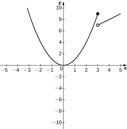
33) $f(x)=\begin{cases}x^2, & x≤3\\ x+4, & x>3\end{cases}$

a. $\displaystyle \lim_{x→3^−}f(x)$

b. $\displaystyle \lim_{x→3^+}f(x)$

Answer

$The graph of a piecewise function with two segments. The first is the parabola x^2, which exists for x<=3. The vertex is at the origin, it opens upward, and there is a closed circle at the endpoint (3,9). The second segment is the line x+4, which is a linear function existing for x > 3. There is an open circle at (3, 7), and the slope is 1.$

a. $9$; b.$ 7$

34) $g(x)=\begin{cases}x^3−1, & x≤0\\1, & x>0\end{cases}$

a. $\displaystyle \lim_{x→0^−}g(x)$

b. $\displaystyle \lim_{x→0^+}g(x)$

35) $h(x)=\begin{cases}x^2−2x+1, & x<2\\3−x, & x≥2\end{cases}$

a. $\displaystyle \lim_{x→2^−}h(x)$

b. $\displaystyle \lim_{x→2^+}h(x)$

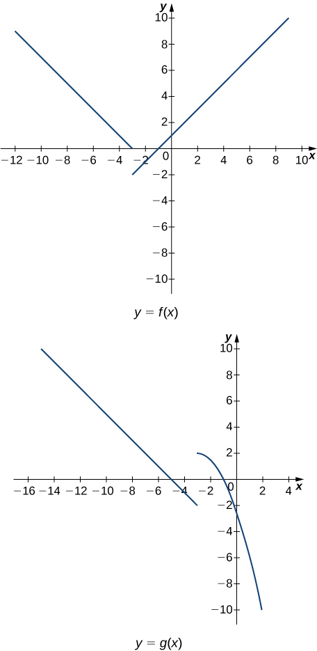
In exercises 36 - 43, use the following graphs and the limit laws to evaluate each limit.

$Two graphs of piecewise functions. The upper is f(x), which has two linear segments. The first is a line with negative slope existing for x < -3. It goes toward the point (-3,0) at x= -3. The next has increasing slope and goes to the point (-3,-2) at x=-3. It exists for x > -3. Other key points are (0, 1), (-5,2), (1,2), (-7, 4), and (-9,6). The lower piecewise function has a linear segment and a curved segment. The linear segment exists for x < -3 and has decreasing slope. It goes to (-3,-2) at x=-3. The curved segment appears to be the right half of a downward opening parabola. It goes to the vertex point (-3,2) at x=-3. It crosses the y axis a little below y=-2. Other key points are (0, -7/3), (-5,0), (1,-5), (-7, 2), and (-9, 4).$

36) $\displaystyle \lim_{x→−3^+}(f(x)+g(x))$

37) $\displaystyle \lim_{x→−3^−}(f(x)−3g(x))$

Answer: $\displaystyle \lim_{x→−3^−}(f(x)−3g(x))=\lim_{x→−3^−}f(x)−3\lim_{x→−3^−}g(x)=0+6=6$

38) $\displaystyle \lim_{x→0}\frac{f(x)g(x)}{3}$

39) $\displaystyle \lim_{x→−5}\frac{2+g(x)}{f(x)}$

Answer: $\displaystyle \lim_{x→−5}\frac{2+g(x)}{f(x)}=\frac{2+\left(\displaystyle \lim_{x→−5}g(x)\right)}{\displaystyle \lim_{x→−5}f(x)}=\frac{2+0}{2}=1$

40) $\displaystyle \lim_{x→1}(f(x))^2$

41) $\displaystyle \lim_{x→1}\sqrt[3]{f(x)−g(x)}$

Answer: $\displaystyle \lim_{x→1}\sqrt[3]{f(x)−g(x)}=\sqrt[3]{\lim_{x→1}f(x)−\lim_{x→1}g(x)}=\sqrt[3]{2+5}=\sqrt[3]{7}$

42) $\displaystyle \lim_{x→−7}(x⋅g(x))$

43) $\displaystyle \lim_{x→−9}[x⋅f(x)+2⋅g(x)]$

Answer: $\displaystyle \lim_{x→−9}(xf(x)+2g(x))=\left(\lim_{x→−9}x\right)\left(\lim_{x→−9}f(x)\right)+2\lim_{x→−9}g(x)=(−9)(6)+2(4)=−46$

For exercises 44 - 46, evaluate the limit using the squeeze theorem. Use a calculator to graph the functions $f(x)$, $g(x)$, and $h(x)$ when possible.

44) [T] True or False? If $2x−1≤g(x)≤x^2−2x+3$, then $\displaystyle \lim_{x→2}g(x)=0$.

45) [T] $\displaystyle \lim_{θ→0}θ^2\cos\left(\frac{1}{θ}\right)$

Answer

The limit is zero.

$The graph of three functions over the domain [-1,1], colored red, green, and blue as follows: red: theta^2, green: theta^2 * cos (1/theta), and blue: - (theta^2). The red and blue functions open upwards and downwards respectively as parabolas with vertices at the origin. The green function is trapped between the two.$

46) $\displaystyle \lim_{x→0}f(x)$, where $f(x)=\begin{cases}0, & x\text{ rational}\\ x^2, & x\text{ irrrational}\end{cases}$

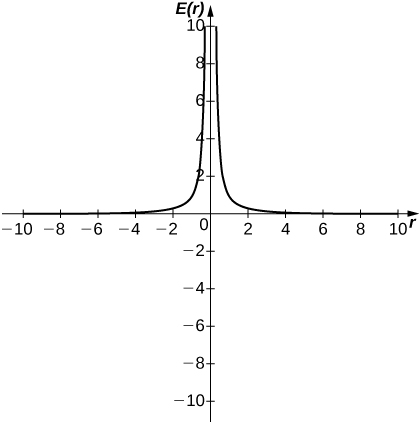
47) [T] In physics, the magnitude of an electric field generated by a point charge at a distance $r$ in vacuum is governed by Coulomb’s law: $E(r)=\dfrac{q}{4πε_0r^2}$, where $E$ represents the magnitude of the electric field, $q$ is the charge of the particle, $r$ is the distance between the particle and where the strength of the field is measured, and $\dfrac{1}{4πε_0}$ is Coulomb’s constant: $8.988×109N⋅m^2/C^2$.

a. Use a graphing calculator to graph $E(r)$ given that the charge of the particle is $q=10^{−10}$.

b. Evaluate $\displaystyle \lim_{r→0^+}E(r)$. What is the physical meaning of this quantity? Is it physically relevant? Why are you evaluating from the right?

Answer

$A graph of a function with two curves. The first is in quadrant two and curves asymptotically to infinity along the y axis and to 0 along the x axis as x goes to negative infinity. The second is in quadrant one and curves asymptotically to infinity along the y axis and to 0 along the x axis as x goes to infinity.$

b. ∞. The magnitude of the electric field as you approach the particle q becomes infinite. It does not make physical sense to evaluate negative distance.

48) [T] The density of an object is given by its mass divided by its volume: $ρ=m/V.$

a. Use a calculator to plot the volume as a function of density $(V=m/ρ)$, assuming you are examining something of mass $8$ kg ($m=8$).

b. Evaluate $\displaystyle \lim_{x→0^+}V(\rho)$ and explain the physical meaning.

Search

Text Color

Text Size

Margin Size

Font Type