Mathematics LibreTexts

4.6E: Exercises for Section 4.6

  • Page ID
    112085
  • \( \newcommand{\vecs}[1]{\overset { \scriptstyle \rightharpoonup} {\mathbf{#1}} } \)

    \( \newcommand{\vecd}[1]{\overset{-\!-\!\rightharpoonup}{\vphantom{a}\smash {#1}}} \)

    \( \newcommand{\id}{\mathrm{id}}\) \( \newcommand{\Span}{\mathrm{span}}\)

    ( \newcommand{\kernel}{\mathrm{null}\,}\) \( \newcommand{\range}{\mathrm{range}\,}\)

    \( \newcommand{\RealPart}{\mathrm{Re}}\) \( \newcommand{\ImaginaryPart}{\mathrm{Im}}\)

    \( \newcommand{\Argument}{\mathrm{Arg}}\) \( \newcommand{\norm}[1]{\| #1 \|}\)

    \( \newcommand{\inner}[2]{\langle #1, #2 \rangle}\)

    \( \newcommand{\Span}{\mathrm{span}}\)

    \( \newcommand{\id}{\mathrm{id}}\)

    \( \newcommand{\Span}{\mathrm{span}}\)

    \( \newcommand{\kernel}{\mathrm{null}\,}\)

    \( \newcommand{\range}{\mathrm{range}\,}\)

    \( \newcommand{\RealPart}{\mathrm{Re}}\)

    \( \newcommand{\ImaginaryPart}{\mathrm{Im}}\)

    \( \newcommand{\Argument}{\mathrm{Arg}}\)

    \( \newcommand{\norm}[1]{\| #1 \|}\)

    \( \newcommand{\inner}[2]{\langle #1, #2 \rangle}\)

    \( \newcommand{\Span}{\mathrm{span}}\) \( \newcommand{\AA}{\unicode[.8,0]{x212B}}\)

    \( \newcommand{\vectorA}[1]{\vec{#1}}      % arrow\)

    \( \newcommand{\vectorAt}[1]{\vec{\text{#1}}}      % arrow\)

    \( \newcommand{\vectorB}[1]{\overset { \scriptstyle \rightharpoonup} {\mathbf{#1}} } \)

    \( \newcommand{\vectorC}[1]{\textbf{#1}} \)

    \( \newcommand{\vectorD}[1]{\overrightarrow{#1}} \)

    \( \newcommand{\vectorDt}[1]{\overrightarrow{\text{#1}}} \)

    \( \newcommand{\vectE}[1]{\overset{-\!-\!\rightharpoonup}{\vphantom{a}\smash{\mathbf {#1}}}} \)

    \( \newcommand{\vecs}[1]{\overset { \scriptstyle \rightharpoonup} {\mathbf{#1}} } \)

    \( \newcommand{\vecd}[1]{\overset{-\!-\!\rightharpoonup}{\vphantom{a}\smash {#1}}} \)

    \(\newcommand{\avec}{\mathbf a}\) \(\newcommand{\bvec}{\mathbf b}\) \(\newcommand{\cvec}{\mathbf c}\) \(\newcommand{\dvec}{\mathbf d}\) \(\newcommand{\dtil}{\widetilde{\mathbf d}}\) \(\newcommand{\evec}{\mathbf e}\) \(\newcommand{\fvec}{\mathbf f}\) \(\newcommand{\nvec}{\mathbf n}\) \(\newcommand{\pvec}{\mathbf p}\) \(\newcommand{\qvec}{\mathbf q}\) \(\newcommand{\svec}{\mathbf s}\) \(\newcommand{\tvec}{\mathbf t}\) \(\newcommand{\uvec}{\mathbf u}\) \(\newcommand{\vvec}{\mathbf v}\) \(\newcommand{\wvec}{\mathbf w}\) \(\newcommand{\xvec}{\mathbf x}\) \(\newcommand{\yvec}{\mathbf y}\) \(\newcommand{\zvec}{\mathbf z}\) \(\newcommand{\rvec}{\mathbf r}\) \(\newcommand{\mvec}{\mathbf m}\) \(\newcommand{\zerovec}{\mathbf 0}\) \(\newcommand{\onevec}{\mathbf 1}\) \(\newcommand{\real}{\mathbb R}\) \(\newcommand{\twovec}[2]{\left[\begin{array}{r}#1 \\ #2 \end{array}\right]}\) \(\newcommand{\ctwovec}[2]{\left[\begin{array}{c}#1 \\ #2 \end{array}\right]}\) \(\newcommand{\threevec}[3]{\left[\begin{array}{r}#1 \\ #2 \\ #3 \end{array}\right]}\) \(\newcommand{\cthreevec}[3]{\left[\begin{array}{c}#1 \\ #2 \\ #3 \end{array}\right]}\) \(\newcommand{\fourvec}[4]{\left[\begin{array}{r}#1 \\ #2 \\ #3 \\ #4 \end{array}\right]}\) \(\newcommand{\cfourvec}[4]{\left[\begin{array}{c}#1 \\ #2 \\ #3 \\ #4 \end{array}\right]}\) \(\newcommand{\fivevec}[5]{\left[\begin{array}{r}#1 \\ #2 \\ #3 \\ #4 \\ #5 \\ \end{array}\right]}\) \(\newcommand{\cfivevec}[5]{\left[\begin{array}{c}#1 \\ #2 \\ #3 \\ #4 \\ #5 \\ \end{array}\right]}\) \(\newcommand{\mattwo}[4]{\left[\begin{array}{rr}#1 \amp #2 \\ #3 \amp #4 \\ \end{array}\right]}\) \(\newcommand{\laspan}[1]{\text{Span}\{#1\}}\) \(\newcommand{\bcal}{\cal B}\) \(\newcommand{\ccal}{\cal C}\) \(\newcommand{\scal}{\cal S}\) \(\newcommand{\wcal}{\cal W}\) \(\newcommand{\ecal}{\cal E}\) \(\newcommand{\coords}[2]{\left\{#1\right\}_{#2}}\) \(\newcommand{\gray}[1]{\color{gray}{#1}}\) \(\newcommand{\lgray}[1]{\color{lightgray}{#1}}\) \(\newcommand{\rank}{\operatorname{rank}}\) \(\newcommand{\row}{\text{Row}}\) \(\newcommand{\col}{\text{Col}}\) \(\renewcommand{\row}{\text{Row}}\) \(\newcommand{\nul}{\text{Nul}}\) \(\newcommand{\var}{\text{Var}}\) \(\newcommand{\corr}{\text{corr}}\) \(\newcommand{\len}[1]{\left|#1\right|}\) \(\newcommand{\bbar}{\overline{\bvec}}\) \(\newcommand{\bhat}{\widehat{\bvec}}\) \(\newcommand{\bperp}{\bvec^\perp}\) \(\newcommand{\xhat}{\widehat{\xvec}}\) \(\newcommand{\vhat}{\widehat{\vvec}}\) \(\newcommand{\uhat}{\widehat{\uvec}}\) \(\newcommand{\what}{\widehat{\wvec}}\) \(\newcommand{\Sighat}{\widehat{\Sigma}}\) \(\newcommand{\lt}{<}\) \(\newcommand{\gt}{>}\) \(\newcommand{\amp}{&}\) \(\definecolor{fillinmathshade}{gray}{0.9}\)

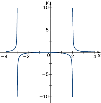
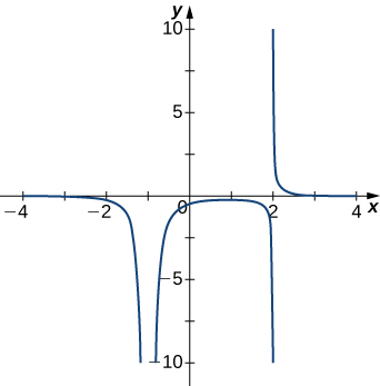
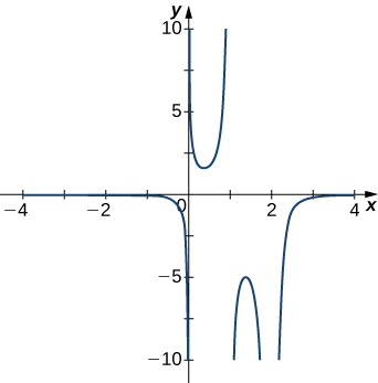
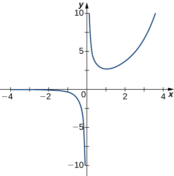
    For exercises 1 - 5, examine the graphs. Identify where the vertical asymptotes are located.

    1)
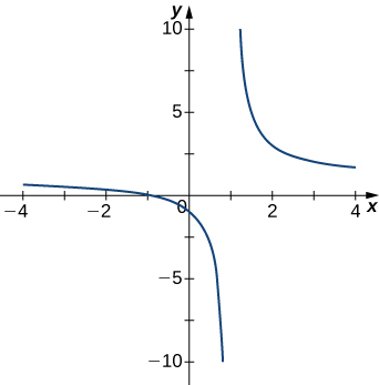
    The function graphed decreases very rapidly as it approaches x = 1 from the left, and on the other side of x = 1, it seems to start near infinity and then decrease rapidly.

    Answer
    \(x=1\)

    2)

    The function graphed increases very rapidly as it approaches x = −3 from the left, and on the other side of x = −3, it seems to start near negative infinity and then increase rapidly to form a sort of U shape that is pointing down, with the other side of the U being at x = 2. On the other side of x = 2, the graph seems to start near infinity and then decrease rapidly.

    3)

    The function graphed decreases very rapidly as it approaches x = −1 from the left, and on the other side of x = −1, it seems to start near negative infinity and then increase rapidly to form a sort of U shape that is pointing down, with the other side of the U being at x = 2. On the other side of x = 2, the graph seems to start near infinity and then decrease rapidly.

    Answer
    \(x=−1,\;x=2\)

    4)

    The function graphed decreases very rapidly as it approaches x = 0 from the left, and on the other side of x = 0, it seems to start near infinity and then decrease rapidly to form a sort of U shape that is pointing up, with the other side of the U being at x = 1. On the other side of x = 1, there is another U shape pointing down, with its other side being at x = 2. On the other side of x = 2, the graph seems to start near negative infinity and then increase rapidly.

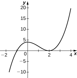
    5)

    The function graphed decreases very rapidly as it approaches x = 0 from the left, and on the other side of x = 0, it seems to start near infinity and then decrease rapidly to form a sort of U shape that is pointing up, with the other side being a normal function that appears as if it will take the entirety of the values of the x-axis.

    Answer
    \(x=0\)

    For the functions \(f(x)\) in exercises 6 - 10, determine whether there is an asymptote at \(x=a\). Justify your answer without graphing on a calculator.

    6) \(f(x)=\dfrac{x+1}{x^2+5x+4},\quad a=−1\)

    7) \(f(x)=\dfrac{x}{x−2},\quad a=2\)

    Answer
    Yes, there is a vertical asymptote at \(x = 2\).

    8) \(f(x)=(x+2)^{3/2},\quad a=−2\)

    9) \(f(x)=(x−1)^{−1/3},\quad a=1\)

    Answer
    Yes, there is vertical asymptote at \(x = 1\).

    10) \(f(x)=1+x^{−2/5},\quad a=1\)

    In exercises 11 - 20, evaluate the limit.

    11) \(\displaystyle \lim_{x→∞}\frac{1}{3x+6}\)

    Answer
    \(\displaystyle \lim_{x→∞}\frac{1}{3x+6} = 0\)

    12) \(\displaystyle \lim_{x→∞}\frac{2x−5}{4x}\)

    13) \(\displaystyle \lim_{x→∞}\frac{x^2−2x+5}{x+2}\)

    Answer
    \(\displaystyle \lim_{x→∞}\frac{x^2−2x+5}{x+2} = ∞\)

    14) \(\displaystyle \lim_{x→−∞}\frac{3x^3−2x}{x^2+2x+8}\)

    15) \(\displaystyle \lim_{x→−∞}\frac{x^4−4x^3+1}{2−2x^2−7x^4}\)

    Answer
    \(\displaystyle \lim_{x→−∞}\frac{x^4−4x^3+1}{2−2x^2−7x^4} = −\frac{1}{7}\)

    16) \(\displaystyle \lim_{x→∞}\frac{3x}{\sqrt{x^2+1}}\)

    17) \(\displaystyle \lim_{x→−∞}\frac{\sqrt{4x^2−1}}{x+2}\)

    Answer
    \(\displaystyle \lim_{x→−∞}\frac{\sqrt{4x^2−1}}{x+2} = -2\)

    18) \(\displaystyle \lim_{x→∞}\frac{4x}{\sqrt{x^2−1}}\)

    19) \(\displaystyle \lim_{x→−∞}\frac{4x}{\sqrt{x^2−1}}\)

    Answer
    \(\displaystyle \lim_{x→−∞}\frac{4x}{\sqrt{x^2−1}} = -4\)

    20) \(\displaystyle \lim_{x→∞}\frac{2\sqrt{x}}{x−\sqrt{x}+1}\)

    For exercises 21 - 25, find the horizontal and vertical asymptotes.

    21) \(f(x)=x−\dfrac{9}{x}\)

    Answer
    Horizontal: none,
    Vertical: \(x=0\)

    22) \(f(x)=\dfrac{1}{1−x^2}\)

    23) \(f(x)=\dfrac{x^3}{4−x^2}\)

    Answer
    Horizontal: none,
    Vertical: \(x=±2\)

    24) \(f(x)=\dfrac{x^2+3}{x^2+1}\)

    25) \(f(x)=\sin(x)\sin(2x)\)

    Answer
    Horizontal: none,
    Vertical: none

    26) \(f(x)=\cos x+\cos(3x)+\cos(5x)\)

    27) \(f(x)=\dfrac{x\sin(x)}{x^2−1}\)

    Answer
    Horizontal: \(y=0,\)
    Vertical: \(x=±1\)

    28) \(f(x)=\dfrac{x}{\sin(x)}\)

    29) \(f(x)=\dfrac{1}{x^3+x^2}\)

    Answer
    Horizontal: \(y=0,\)
    Vertical: \(x=0\) and \(x=−1\)

    30) \(f(x)=\dfrac{1}{x−1}−2x\)

    31) \(f(x)=\dfrac{x^3+1}{x^3−1}\)

    Answer
    Horizontal: \(y=1,\)
    Vertical: \(x=1\)

    32) \(f(x)=\dfrac{\sin x+\cos x}{\sin x−\cos x}\)

    33) \(f(x)=x−\sin x\)

    Answer
    Horizontal: none,
    Vertical: none

    34) \(f(x)=\dfrac{1}{x}−\sqrt{x}\)

    For exercises 35 - 38, construct a function \(f(x)\) that has the given asymptotes.

    35) \(x=1\) and \(y=2\)

    Answer
    Answers will vary, for example: \(y=\dfrac{2x}{x−1}\)

    36) \(x=1\) and \(y=0\)

    37) \(y=4, \;x=−1\)

    Answer
    Answers will vary, for example: \(y=\dfrac{4x}{x+1}\)

    38) \(x=0\)

    In exercises 39 - 43, graph the function on a graphing calculator on the window \(x=[−5,5]\) and estimate the horizontal asymptote or limit. Then, calculate the actual horizontal asymptote or limit.

    39) [T] \(f(x)=\dfrac{1}{x+10}\)

    Answer
    \(\displaystyle \lim_{x→∞}\frac{1}{x+10}=0\) so \(f\) has a horizontal asymptote of \(y=0\).

    40) [T] \(f(x)=\dfrac{x+1}{x^2+7x+6}\)

    41) [T] \(\displaystyle \lim_{x→−∞}x^2+10x+25\)

    Answer
    \(\displaystyle \lim_{x→−∞}x^2+10x+25 = ∞\)

    42) [T] \(\displaystyle \lim_{x→−∞}\frac{x+2}{x^2+7x+6}\)

    43) [T] \(\displaystyle \lim_{x→∞}\frac{3x+2}{x+5}\)

    Answer
    \(\displaystyle \lim_{x→∞}\frac{3x+2}{x+5}=3\) so this function has a horizontal asymptote of \(y=3\).

    In exercises 44 - 55, draw a graph of the functions without using a calculator. Be sure to notice all important features of the graph: local maxima and minima, inflection points, and asymptotic behavior.

    44) \(y=3x^2+2x+4\)

    45) \(y=x^3−3x^2+4\)

    Answer
    The function starts in the third quadrant, increases to pass through (−1, 0), increases to a maximum and y intercept at 4, decreases to touch (2, 0), and then increases to (4, 20).

    46) \(y=\dfrac{2x+1}{x^2+6x+5}\)

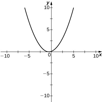
    47) \(y=\dfrac{x^3+4x^2+3x}{3x+9}\)

    Answer
    An upward-facing parabola with minimum between x = 0 and x = −1 with y intercept between 0 and 1.

    48) \(y=\dfrac{x^2+x−2}{x^2−3x−4}\)

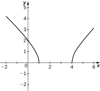
    49) \(y=\sqrt{x^2−5x+4}\)

    Answer
    This graph starts at (−2, 4) and decreases in a convex way to (1, 0). Then the graph starts again at (4, 0) and increases in a convex way to (6, 3).

    50) \(y=2x\sqrt{16−x^2}\)

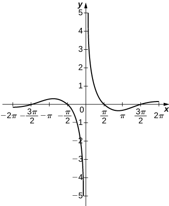
    51) \(y=\dfrac{\cos x}{x}\), on \(x=[−2π,2π]\)

    Answer
    This graph has vertical asymptote at x = 0. The first part of the function occurs in the second and third quadrants and starts in the third quadrant just below (−2π, 0), increases and passes through the x axis at −3π/2, reaches a maximum and then decreases through the x axis at −π/2 before approaching the asymptote. On the other side of the asymptote, the function starts in the first quadrant, decreases quickly to pass through π/2, decreases to a local minimum and then increases through (3π/2, 0) before staying just above (2π, 0).

    52) \(y=e^x−x^3\)

    53) \(y=x\tan x, \quad x=[−π,π]\)

    Answer
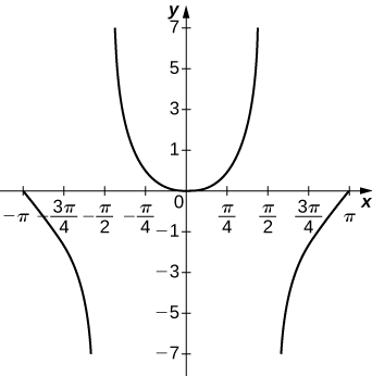
    This graph has vertical asymptotes at x = ±π/2. The graph is symmetric about the y axis, so describing the left hand side will be sufficient. The function starts at (−π, 0) and decreases quickly to the asymptote. Then it starts on the other side of the asymptote in the second quadrant and decreases to the the origin.

    54) \(y=x\ln(x), \quad x>0\)

    55) \(y=x^2\sin(x),\quad x=[−2π,2π]\)

    Answer
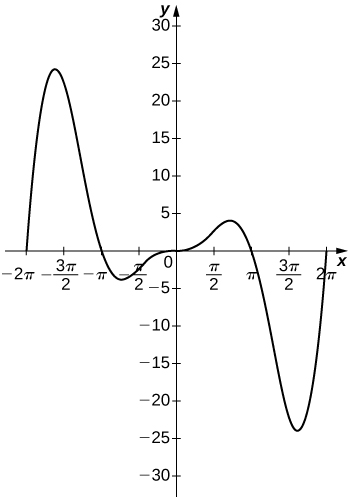
    This function starts at (−2π, 0), increases to near (−3π/2, 25), decreases through (−π, 0), achieves a local minimum and then increases through the origin. On the other side of the origin, the graph is the same but flipped, that is, it is congruent to the other half by a rotation of 180 degrees.

    56) For \(f(x)=\dfrac{P(x)}{Q(x)}\) to have an asymptote at \(y=2\) then the polynomials \(P(x)\) and \(Q(x)\) must have what relation?

    57) For \(f(x)=\dfrac{P(x)}{Q(x)}\) to have an asymptote at \(x=0\), then the polynomials \(P(x)\) and \(Q(x).\) must have what relation?

    Answer
    \(Q(x).\) must have have \(x^{k+1}\) as a factor, where \(P(x)\) has \(x^k\) as a factor.

    58) If \(f′(x)\) has asymptotes at \(y=3\) and \(x=1\), then \(f(x)\) has what asymptotes?

    59) Both \(f(x)=\dfrac{1}{x−1}\) and \(g(x)=\dfrac{1}{(x−1)^2}\) have asymptotes at \(x=1\) and \(y=0.\) What is the most obvious difference between these two functions?

    Answer
    \(\displaystyle \lim_{x→1^−}f(x)=-\infty \text{ and } \lim_{x→1^−}g(x)=\infty\)

    60) True or false: Every ratio of polynomials has vertical asymptotes.


    4.6E: Exercises for Section 4.6 is shared under a not declared license and was authored, remixed, and/or curated by LibreTexts.

    • Was this article helpful?