15.1E: Exercises for Section 15.1

In exercises 1 and 2, use the midpoint rule with \(m = 4\) and \(n = 2\) to estimate the volume of the solid bounded by the surface \(z = f(x,y)\), the vertical planes \(x = 1\), \(x = 2\), \(y = 1\), and \(y = 2\), and the horizontal plane \(x = 0\).

1) \(f(x,y) = 4x + 2y + 8xy\)

Answer

\(27\)

2) \(f(x,y) = 16x^2 + \frac{y}{2}\)

In Exercises 3 and 4, a graph of a planar region \(R\) is given. Give the iterated integrals, with both orders of integration \(dy\,dx\) and \(dx\,dy\), that give the area of \(R\). Evaluate one of the iterated integrals to find the area.

3.

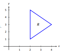
Answer

\( \text{Area} = \displaystyle \quad 4 \,\text{units}^2\)

4.

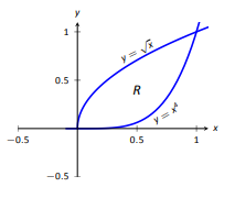
Answer

\( \text{Area} = \displaystyle \quad \dfrac{7}{15} \,\text{units}^2\)

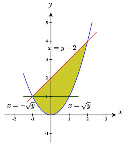
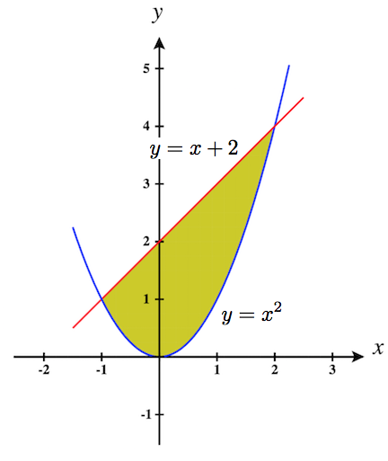
In Exercise 5, iterated integrals are given that compute the area of a region R in the xy-plane. Sketch the region R, and give the iterated integral(s) that give the area of R with the opposite order of integration.

5. \(\displaystyle \int_{0}^1 \int_{-\sqrt{y}}^{\sqrt{y}}\,dx\,dy +\int_1^4 \int_{y-2}^{\sqrt{y}}\,dx\,dy\)

Answer

\(\displaystyle \int_{0}^1 \int_{-\sqrt{y}}^{\sqrt{y}}\,dx\,dy +\int_1^4 \int_{y-2}^{\sqrt{y}}\,dx\,dy \quad\) \(=\quad \displaystyle \int_{-1}^2 \int_{x^2}^{x+2}\,dy\,dx\)

6) The values of the function \(f\) on the rectangle \(R = [0,2] \times [7,9]\) are given in the following table. Estimate the double integral \(\iint_R f(x,y)\,dA\) by using a Riemann sum with \(m = n = 2\). Select the sample points to be the upper right corners of the sub-squares of R.

	\(y_0 = 7\)	\(y_1 = 8\)	\(y_2 = 9\)
\(x_0 = 0\)	10.22	10.21	9.85
\(x_1 = 1\)	6.73	9.75	9.63
\(x_2 = 2\)	5.62	7.83	8.21

7) The depth of a children’s 4-ft by 4-ft swimming pool, measured at 1-ft intervals, is given in the following table.

1. Estimate the volume of water in the swimming pool by using a Riemann sum with \(m = n = 2\). Select the sample points using the midpoint rule on \(R = [0,4] \times [0,4]\).
2. Find the average depth of the swimming pool.

   	\(y\)
   \(x\)	0	1	2	3	4
   0	1	1.5	2	2.5	3
   1	1	1.5	2	2.5	3
   2	1	1.5	1.5	2.5	3
   3	1	1	1.5	2	2.5
   4	1	1	1	1.5	2

Answer

a. 28 \(\text{ft}^3\)
b. 1.75 ft.

8) The depth of a 3-ft by 3-ft hole in the ground, measured at 1-ft intervals, is given in the following table.

1. Estimate the volume of the hole by using a Riemann sum with \(m = n = 3\) and the sample points to be the upper left corners of the sub-squares of \(R\).
2. Find the average depth of the hole.

   	\(y\)
   \(x\)	0	1	2	3
   0	6	6.5	6.4	6
   1	6.5	7	7.5	6.5
   2	6.5	6.7	6.5	6
   3	6	6.5	5	5.6

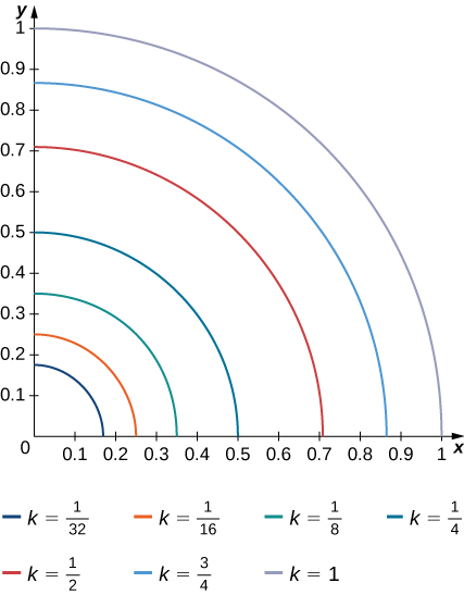
9) The level curves \(f(x,y) = k\) of the function \(f\) are given in the following graph, where \(k\) is a constant.

1. Apply the midpoint rule with \(m = n = 2\) to estimate the double integral \(\iint_R f(x,y)\,dA\), where \(R = [0.2,1] \times [0,0.8]\).
2. Estimate the average value of the function \(f\) on \(R\).

   

Answer

a. 0.112
b. \(f_{ave} ≃ 0.175\); here \(f(0.4,0.2) ≃ 0.1\), \(f(0.2,0.6) ≃− 0.2\), \(f(0.8,0.2) ≃ 0.6\), and \(f(0.8,0.6) ≃ 0.2\)

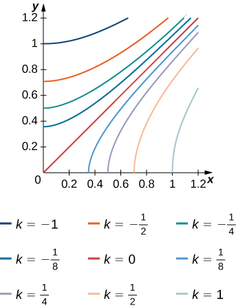
10) The level curves \(f(x,y) = k\) of the function \(f\) are given in the following graph, where \(k\) is a constant.

1. Apply the midpoint rule with \(m = n = 2\) to estimate the double integral \(\iint_R f(x,y)\,dA\), where \(R = [0.1,0.5] \times [0.1,0.5]\).
2. Estimate the average value of the function f on \(R\).

   

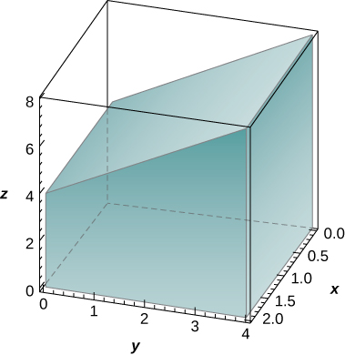
11) The solid lying under the surface \(z = \sqrt{4 - y^2}\) and above the rectangular region\( R = [0,2] \times [0,2]\) is illustrated in the following graph. Evaluate the double integral \(\iint_Rf(x,y)\), where \(f(x,y) = \sqrt{4 - y^2}\) by finding the volume of the corresponding solid. Hint: Use the volume formula for a cylinder, don't actually do the integral.

Answer

\(2\pi\)

12) The solid lying under the plane \(z = y + 4\) and above the rectangular region \(R = [0,2] \times [0,4]\) is illustrated in the following graph. Evaluate the double integral \(\iint_R f(x,y)\,dA\), where \(f(x,y) = y + 4\), by finding the volume of the corresponding solid. Hint: Use volume formulas, don't actually do the integral.

Answer

\(48\)

In the exercises 13 - 20, calculate the integrals by reversing the order of integration.

13) \(\displaystyle \int_{-1}^1\left(\int_{-2}^2 (2x + 3y + 5)\,dx \right) \space dy\)

Answer

\(40\)

14) \(\displaystyle \int_0^2\left(\int_0^1 (x + 2e^y + 3)\,dx \right) \space dy\)

15) \(\displaystyle \int_1^{27}\left(\int_1^2 (\sqrt[3]{x} + \sqrt[3]{y})\,dy \right) \space dx\)

Answer

\(\frac{81}{2} + 39\sqrt[3]{2}\)

16) \(\displaystyle \int_1^{16}\left(\int_1^8 (\sqrt[4]{x} + 2\sqrt[3]{y})\,dy \right) \space dx\)

17) \(\displaystyle \int_{\ln 2}^{\ln 3}\left(\int_0^1 e^{x+y}\,dy \right) \space dx\)

Answer

\(e - 1\)

18) \(\displaystyle \int_0^2\left(\int_0^1 3^{x+y}\,dy \right) \space dx\)

19) \(\displaystyle \int_1^6\left(\int_2^9 \frac{\sqrt{y}}{x^2}\,dy \right) \space dx\)

Answer

\(15 - \frac{10\sqrt{2}}{9}\)

20) \(\displaystyle \int_1^9 \left(\int_4^2 \frac{\sqrt{x}}{y^2}\,dy \right)\,dx\)

In exercises 21 - 34, evaluate the iterated integrals by choosing the order of integration.

21) \(\displaystyle \int_0^{\pi} \int_0^{\pi/2} \sin(2x)\cos(3y)\,dx \space dy\)

Answer

\(0\)

22) \(\displaystyle \int_{\pi/12}^{\pi/8}\int_{\pi/4}^{\pi/3} [\cot x + \tan(2y)]\,dx \space dy\)

23) \(\displaystyle \int_1^e \int_1^e \left[\frac{1}{x}\sin(\ln x) + \frac{1}{y}\cos (\ln y)\right] \,dx \space dy\)

Answer

\((e − 1)(1 + \sin 1 − \cos 1)\)

24) \(\displaystyle \int_1^e \int_1^e \frac{\sin(\ln x)\cos (\ln y)}{xy} \,dx \space dy\)

25) \(\displaystyle \int_1^2 \int_1^2 \left(\frac{\ln y}{x} + \frac{x}{2y + 1}\right)\,dy \space dx\)

Answer

\(\frac{3}{4}\ln \left(\frac{5}{3}\right) + 2 (\ln 2)^2 - \ln 2\)

26) \(\displaystyle \int_1^e \int_1^2 x^2 \ln(x)\,dy \space dx\)

27) \(\displaystyle \int_1^{\sqrt{3}} \int_1^2 y \space \arctan \left(\frac{1}{x}\right) \,dy \space dx\)

Answer

\(\frac{1}{8}[(2\sqrt{3} - 3) \pi + 6 \space \ln 2]\)

28) \(\displaystyle \int_0^1 \int_0^{1/2} (\arcsin x + \arcsin y)\,dy \space dx\)

29) \(\displaystyle \int_0^1 \int_1^2 xe^{x+4y}\,dy \space dx\)

Answer

\(\frac{1}{4}e^4 (e^4 - 1)\)

30) \(\displaystyle \int_1^2 \int_0^1 xe^{x-y}\,dy \space dx\)

31) \(\displaystyle \int_1^2 \int_1^x (x^2y-y+2)\,dy\,dx\)

Answer

\(\displaystyle \quad \dfrac{34}{15}\)

32) \(\displaystyle \int_0^{\pi} \int_0^{y} (\cos x \sin y)\,dx\,dy\)

Answer

\(\displaystyle \quad \dfrac{\pi}{2}\)

33) \(\displaystyle \int_0^1 \int_1^2 \left(\frac{x}{x^2 + y^2} \right)\,dy \space dx\)

Answer

\(-\frac{\pi}{4} + \ln \left(\frac{5}{4}\right) - \frac{1}{2} \ln 2 + \arctan 2\)

34) \(\displaystyle \int_0^1 \int_1^2 \frac{y}{x + y^2}\,dy \space dx\)

In exercises 35 - 38, find the average value of the function over the given rectangles.

35)\(f(x,y) = −x +2y\), \(R = [0,1] \times [0,1]\)

Answer

\(\frac{1}{2}\)

36) \(f(x,y) = x^4 + 2y^3\), \(R = [1,2] \times [2,3]\)

37) \(f(x,y) = \sinh x + \sinh y\), \(R = [0,1] \times [0,2]\)

Answer

\(\frac{1}{2}(2 \space \cosh 1 + \cosh 2 - 3)\).

38) \(f(x,y) = \arctan(xy)\), \(R = [0,1] \times [0,1]\)

39) Let \(f\) and \(g\) be two continuous functions such that \(0 \leq m_1 \leq f(x) \leq M_1\) for any \(x ∈ [a,b]\) and \(0 \leq m_2 \leq g(y) \leq M_2\) for any\( y ∈ [c,d]\). Show that the following inequality is true:

\[m_1m_2(b-a)(c-d) \leq \int_a^b \int_c^d f(x) g(y)\,dy dx \leq M_1M_2 (b-a)(c-d). \nonumber \]

In exercises 40 - 43, use property v. of double integrals and the answer from the preceding exercise to show that the following inequalities are true.

40) \(\frac{1}{e^2} \leq \iint_R e^{-x^2 - y^2} \space dA \leq 1\), where \(R = [0,1] \times [0,1]\)

41) \(\frac{\pi^2}{144} \leq \iint_R \sin x \cos y \space dA \leq \frac{\pi^2}{48}\), where \(R = \left[ \frac{\pi}{6}, \frac{\pi}{3}\right] \times \left[ \frac{\pi}{6}, \frac{\pi}{3}\right]\)

42) \(0 \leq \iint_R e^{-y}\space \cos x \space dA \leq \frac{\pi}{2}\), where \(R = \left[0, \frac{\pi}{2}\right] \times \left[0, \frac{\pi}{2}\right]\)

43) \(0 \leq \iint_R (\ln x)(\ln y) \,dA \leq (e - 1)^2\), where \(R = [1, e] \times [1, e] \)

44) Let \(f\) and \(g\) be two continuous functions such that \(0 \leq m_1 \leq f(x) \leq M_1\) for any \(x ∈ [a,b]\) and \(0 \leq m_2 \leq g(y) \leq M_2\) for any \(y ∈ [c,d]\). Show that the following inequality is true:

\[(m_1 + m_2) (b - a)(c - d) \leq \int_a^b \int_c^d |f(x) + g(y)| \space dy \space dx \leq (M_1 + M_2)(b - a)(c - d) \nonumber \]

In exercises 45 - 48, use property v. of double integrals and the answer from the preceding exercise to show that the following inequalities are true.

45) \(\frac{2}{e} \leq \iint_R (e^{-x^2} + e^{-y^2}) \,dA \leq 2\), where \(R = [0,1] \times [0,1]\)

46) \(\frac{\pi^2}{36}\iint_R (\sin x + \cos y)\,dA \leq \frac{\pi^2 \sqrt{3}}{36}\), where \(R = [\frac{\pi}{6}, \frac{\pi}{3}] \times [\frac{\pi}{6}, \frac{\pi}{3}]\)

47) \(\frac{\pi}{2}e^{-\pi/2} \leq \iint_R (\cos x + e^{-y})\,dA \leq \pi\), where \(R = [0, \frac{\pi}{2}] \times [0, \frac{\pi}{2}]\)

48) \(\frac{1}{e} \leq \iint_R (e^{-y} - \ln x) \,dA \leq 2\), where \(R = [0, 1] \times [0, 1]\)

In exercises 49 - 50, the function \(f\) is given in terms of double integrals.

1. Determine the explicit form of the function \(f\).
2. Find the volume of the solid under the surface \(z = f(x,y)\) and above the region \(R\).
3. Find the average value of the function \(f\) on \(R\).
4. Use a computer algebra system (CAS) to plot \(z = f(x,y)\) and \(z = f_{ave}\) in the same system of coordinates.

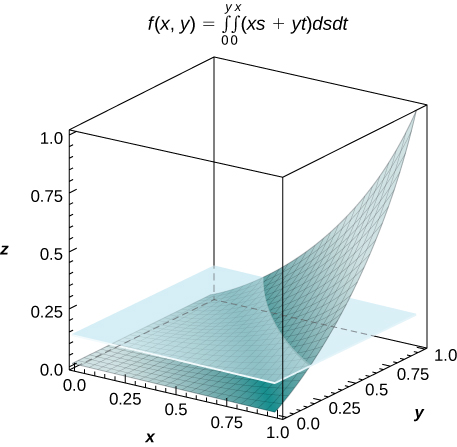
49) [T] \(f(x,y) = \int_0^y \int_0^x (xs + yt) ds \space dt\), where \((x,y) \in R = [0,1] \times [0,1]\)

Answer

a. \(f(x,y) = \frac{1}{2} xy (x^2 + y^2)\);
b. \(V = \int_0^1 \int_0^1 f(x,y)\,dx \space dy = \frac{1}{8}\);
c. \(f_{ave} = \frac{1}{8}\);

d.

50) [T] \(f(x,y) = \int_0^x \int_0^y [\cos(s) + \cos(t)] \, dt \space ds\), where \((x,y) \in R = [0,3] \times [0,3]\)

51) Show that if \(f\) and \(g\) are continuous on \([a,b]\) and \([c,d]\), respectively, then

\(\displaystyle \int_a^b \int_c^d |f(x) + g(y)| dy \space dx = (d - c) \int_a^b f(x)\,dx\)

\(\displaystyle + \int_a^b \int_c^d g(y)\,dy \space dx = (b - a) \int_c^d g(y)\,dy + \int_c^d \int_a^b f(x)\,dx \space dy\).

52) Show that \(\displaystyle \int_a^b \int_c^d yf(x) + xg(y)\,dy \space dx = \frac{1}{2} (d^2 - c^2) \left(\int_a^b f(x)\,dx\right) + \frac{1}{2} (b^2 - a^2) \left(\int_c^d g(y)\,dy\right)\).

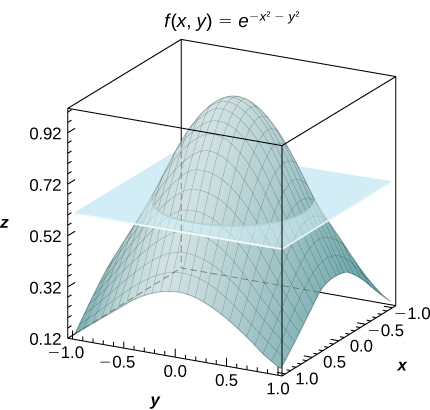
53) [T] Consider the function \(f(x,y) = e^{-x^2-y^2}\), where \((x,y) \in R = [−1,1] \times [−1,1]\).

1. Use the midpoint rule with \(m = n = 2,4,..., 10\) to estimate the double integral \(I = \iint_R e^{-x^2 - y^2} dA\). Round your answers to the nearest hundredths.
2. For \(m = n = 2\), find the average value of f over the region R. Round your answer to the nearest hundredths.
3. Use a CAS to graph in the same coordinate system the solid whose volume is given by \(\iint_R e^{-x^2-y^2} dA\) and the plane \(z = f_{ave}\).

Answer

a. For \(m = n = 2\), \(I = 4e^{-0.5} \approx 2.43\)
b. \(f_{ave} = e^{-0.5} \simeq 0.61\);

c.

54) [T] Consider the function \(f(x,y) = \sin (x^2) \space \cos (y^2)\), where \((x,y \in R = [−1,1] \times [−1,1]\).

1. Use the midpoint rule with \(m = n = 2,4,..., 10\) to estimate the double integral \(I = \iint_R \sin (x^2) \cos (y^2) \space dA\). Round your answers to the nearest hundredths.
2. For \(m = n = 2\), find the average value of \(f\)over the region R. Round your answer to the nearest hundredths.
3. Use a CAS to graph in the same coordinate system the solid whose volume is given by \(\iint_R \sin(x^2) \cos(y^2) \space dA\) and the plane \(z = f_{ave}\).

In exercises 55 - 56, the functions \(f_n\) are given, where \(n \geq 1\) is a natural number.

1. Find the volume of the solids \(S_n\) under the surfaces \(z = f_n(x,y)\) and above the region \(R\).
2. Determine the limit of the volumes of the solids \(S_n\) as \(n\) increases without bound.

55) \(f(x,y) = x^n + y^n + xy, \space (x,y) \in R = [0,1] \times [0,1]\)

Answer

a. \(\frac{2}{n + 1} + \frac{1}{4}\)
b. \(\frac{1}{4}\)

56) \(f(x,y) = \frac{1}{x^n} + \frac{1}{y^n}, \space (x,y) \in R = [1,2] \times [1,2]\)

57) Show that the average value of a function \(f\) on a rectangular region \(R = [a,b] \times [c,d]\) is \(f_{ave} \approx \frac{1}{mn} \sum_{i=1}^m \sum_{j=1}^n f(x_{ij}^*,y_{ij}^*)\),where \((x_{ij}^*,y_{ij}^*)\) are the sample points of the partition of \(R\), where \(1 \leq i \leq m\) and \(1 \leq j \leq n\).

58) Use the midpoint rule with \(m = n\) to show that the average value of a function \(f\) on a rectangular region \(R = [a,b] \times [c,d]\) is approximated by

\[f_{ave} \approx \frac{1}{n^2} \sum_{i,j =1}^n f \left(\frac{1}{2} (x_{i=1} + x_i), \space \frac{1}{2} (y_{j=1} + y_j)\right). \nonumber \]

59) An isotherm map is a chart connecting points having the same temperature at a given time for a given period of time. Use the preceding exercise and apply the midpoint rule with \(m = n = 2\) to find the average temperature over the region given in the following figure.

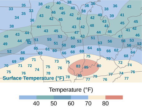
Answer

\(56.5^{\circ}\) F; here \(f(x_1^*,y_1^*) = 71, \space f(x_2^*, y_1^*) = 72, \space f(x_2^*,y_1^*) = 40, \space f(x_2^*,y_2^*) = 43\), where \(x_i^*\) and \(y_j^*\) are the midpoints of the subintervals of the partitions of \([a,b]\) and \([c,d]\), respectively.