7.4: Vectors in Three Dimensions

Learning Objectives 

• Locate points in space using coordinates.
• Write the distance formula in three dimensions.
• Perform vector operations in \(\mathbb{R}^{3}\).

Vectors are useful tools for solving two-dimensional problems. Life, however, happens in three dimensions. To expand the use of vectors to more realistic applications, it is necessary to create a framework for describing three-dimensional space. For example, although a two-dimensional map is a useful tool for navigating from one place to another, in some cases the topography of the land is important. Does your planned route go through the mountains? Do you have to cross a river? To appreciate fully the impact of these geographic features, you must use three dimensions. This section presents a natural extension of the two-dimensional Cartesian coordinate plane into three dimensions.

Three-Dimensional Coordinate Systems

As we have learned, the two-dimensional rectangular coordinate system contains two perpendicular axes: the horizontal \(x\)-axis and the vertical \(y\)-axis. We can add a third dimension, the \(z\)-axis, which is perpendicular to both the \(x\)-axis and the \(y\)-axis. We call this system the three-dimensional rectangular coordinate system. It represents the three dimensions we encounter in real life.

Definition: Three-dimensional Rectangular Coordinate System

The three-dimensional rectangular coordinate system consists of three perpendicular axes: the \(x\)-axis, the \(y\)-axis, and the \(z\)-axis. Because each axis is a number line representing all real numbers in \(ℝ\), the three-dimensional system is often denoted by \(ℝ^3\).

In Figure \(\PageIndex{1a}\), the positive \(z\)-axis is shown above the plane containing the \(x\)- and \(y\)-axes. The positive \(x\)-axis appears to the left and the positive \(y\)-axis is to the right. A natural question to ask is: How was this arrangement determined? The system displayed follows the right-hand rule. If we take our right hand and align the fingers with the positive \(x\)-axis, then curl the fingers so they point in the direction of the positive \(y\)-axis, our thumb points in the direction of the positive \(z\)-axis (Figure \(\PageIndex{1b}\)). In this text, we always work with coordinate systems set up in accordance with the right-hand rule. Some systems do follow a left-hand rule, but the right-hand rule is considered the standard representation.

Figure \(\PageIndex{1}\): (a) We can extend the two-dimensional rectangular coordinate system by adding a third axis, the \(z\)-axis, that is perpendicular to both the \(x\)-axis and the \(y\)-axis. (b) The right-hand rule is used to determine the placement of the coordinate axes in the standard Cartesian plane.

In two dimensions, we describe a point in the plane with the coordinates \((x,y)\). Each coordinate describes how the point aligns with the corresponding axis. In three dimensions, a new coordinate, \(z\), is appended to indicate alignment with the \(z\)-axis: \((x,y,z)\). A point in space is identified by all three coordinates (Figure \(\PageIndex{2}\)). To plot the point \((x,y,z)\), go \(x\) units along the \(x\)-axis, then \(y\) units in the direction of the \(y\)-axis, then \(z\) units in the direction of the \(z\)-axis.

Figure \(\PageIndex{2}\): To plot the point \((x,y,z)\) go \(x\) units along the \(x\)-axis, then \(y\) units in the direction of the \(y\)-axis, then \(z\) units in the direction of the \(z\)-axis.

Example \(\PageIndex{1}\): Locating Points in Space

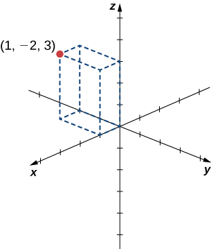
Sketch the point \((1,−2,3)\) in three-dimensional space.

Solution

To sketch a point, start by sketching three sides of a rectangular prism along the coordinate axes: one unit in the positive \(x\) direction, \(2\) units in the negative \(y\) direction, and \(3\) units in the positive \(z\) direction. Complete the prism to plot the point (Figure 3).

Figure \(\PageIndex{3}\): Sketching the point \((1,−2,3).\)

Try It \(\PageIndex{1}\)

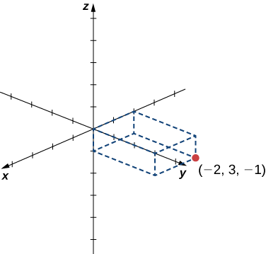
Sketch the point \((−2,3,−1)\) in three-dimensional space.

Hint Start by sketching the coordinate axes. e.g., Figure \(\PageIndex{3b}\). Then sketch a rectangular prism to help find the point in space.

Answer

Most work in three-dimensional space is a comfortable extension of the corresponding concepts in two dimensions. We begin by adapting the distance formula to three-dimensional space.

If two points lie in the same coordinate plane, then it is straightforward to calculate the distance between them. We that the distance \(d\) between two points \((x_1,y_1)\) and \((x_2,y_2)\) in the x\(y\)-coordinate plane is given by the formula

\(d=\sqrt{(x_2−x_1)^2+(y_2−y_1)^2}.\)

The formula for the distance between two points in space is a natural extension of this formula.

Definition: The Distance between Two Points in Space

The distance \(d\) between points \((x_1,y_1,z_1)\) and \((x_2,y_2,z_2)\) is given by the formula

\(d=\sqrt{(x_2−x_1)^2+(y_2−y_1)^2+(z_2−z_1)^2}. \label{distanceForm}\)

 The proof of this theorem is left as an exercise. (Hint: First find the distance \(d_1\) between the points \((x_1,y_1,z_1)\) and \((x_2,y_2,z_1)\) as shown in Figure \(\PageIndex{4}\).

Figure \(\PageIndex{4}\): The distance between \(P_1\) and \(P_2\) is the length of the diagonal of the rectangular prism having \(P_1\) and \(P_2\) as opposite corners.

Example \(\PageIndex{2}\): Distance in Space

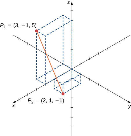
Find the distance between points \(P_1=(3,−1,5)\) and \(P_2=(2,1,−1).\)

Figure \(\PageIndex{5}\): Find the distance between the two points.

Solution

Substitute values directly into the distance formula:

\[\begin{align*} d(P_1,P_2) &=\sqrt{(x_2−x_1)^2+(y_2−y_1)^2+(z_2−z_1)^2} \\[4pt] &=\sqrt{(2−3)^2+(1−(−1))^2+(−1−5)^2} \\[4pt] &=\sqrt{(-1)^2+2^2+(−6)^2}  =\sqrt{41}. \end{align*}\]

 Try It \(\PageIndex{2}\)

Find the distance between points \(P_1=(1,−5,4)\) and \(P_2=(4,−1,−1)\).

Hint

\(d=\sqrt{(x_2−x_1)^2+(y_2−y_1)^2+(z_2−z_1)^2}\)

Answer

\(5\sqrt{2}\)

Working with Vectors in \(ℝ^3\)

Just like two-dimensional vectors, three-dimensional vectors are quantities with both magnitude and direction, and they are represented by directed line segments (arrows). With a three-dimensional vector, we use a three-dimensional arrow.

Three-dimensional vectors can also be represented in component form. The notation \(\vecs{v}=⟨x,y,z⟩\) is a natural extension of the two-dimensional case, representing a vector with the initial point at the origin, \((0,0,0)\), and terminal point \((x,y,z)\). The zero vector is \(\vecs{0}=⟨0,0,0⟩\). So, for example, the three dimensional vector \(\vecs{v}=⟨2,4,1⟩\) is represented by a directed line segment from point \((0,0,0)\) to point \((2,4,1)\) (Figure \(\PageIndex{6}\)).

Figure \(\PageIndex{6}\): Vector \(\vecs{v}=⟨2,4,1⟩\) is represented by a directed line segment from point \((0,0,0)\) to point \((2,4,1).\)

Vector addition and scalar multiplication are defined analogously to the two-dimensional case. If \(\vecs{v}=⟨x_1,y_1,z_1⟩\) and \(\vecs{w}=⟨x_2,y_2,z_2⟩\) are vectors, and \(k\) is a scalar, then

\(\vecs{v}+\vecs{w}=⟨x_1+x_2,y_1⟩+⟨y_2,z_1+z_2⟩\)

and

\(k\vecs{v}=⟨kx_1,ky_1,kz_1⟩.\)

If \(k=−1,\) then \(k\vecs{v}=(−1)\vecs{v}\) is written as \(−\vecs{v}\), and vector subtraction is defined by \(\vecs{v}−\vecs{w}=\vecs{v}+(−\vecs{w})=\vecs{v}+(−1)\vecs{w}\).

The standard unit vectors extend easily into three dimensions as well, \(\hat{\mathbf i}=⟨1,0,0⟩\), \(\hat{\mathbf j}=⟨0,1,0⟩\), and \(\hat{\mathbf k}=⟨0,0,1⟩\), and we use them in the same way we used the standard unit vectors in two dimensions. Thus, we can represent a vector in \(ℝ^3\) in the following ways:

\(\vecs{v}=⟨x,y,z⟩=x\hat{\mathbf i}+y\hat{\mathbf j}+z\hat{\mathbf k}\).

Example \(\PageIndex{3}\): Vector Representations

Figure \(\PageIndex{7}\): The vector with initial point \(P=(3,12,6)\) and terminal point \(Q=(−4,−3,2)\).

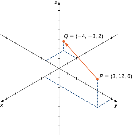
Let \(\vecd{PQ}\) be the vector with initial point \(P=(3,12,6)\) and terminal point \(Q=(−4,−3,2)\) as shown in Figure \(\PageIndex{7}\). Express \(\vecd{PQ}\) in both component form and using standard unit vectors.

Solution

In component form,

\[\begin{align*} \vecd{PQ} =⟨x_2−x_1,y_2−y_1,z_2−z_1⟩ \\[4pt] =⟨−4−3,−3−12,2−6⟩  =⟨−7,−15,−4⟩. \end{align*}\]

In standard unit form,

\[\vecd{PQ}=−7\hat{\mathbf i}−15\hat{\mathbf j}−4\hat{\mathbf k}. \nonumber\]

 Try It \(\PageIndex{3}\)

Let \(S=(3,8,2)\) and \(T=(2,−1,3)\). Express \(\vec{ST}\) in component form and in standard unit form.

Hint

Write \(\vecd{ST}\) in component form first. \(T\) is the terminal point of \(\vecd{ST}\).

Answer

\(\vecd{ST}=⟨−1,−9,1⟩=−\hat{\mathbf i}−9\hat{\mathbf j}+\hat{\mathbf k}\)

As described earlier, vectors in three dimensions behave in the same way as vectors in a plane. The geometric interpretation of vector addition, for example, is the same in both two- and three-dimensional space (Figure \(\PageIndex{8}\)).

Figure \(\PageIndex{8}\): To add vectors in three dimensions, we follow the same procedures we learned for two dimensions.

We have already seen how some of the algebraic properties of vectors, such as vector addition and scalar multiplication, can be extended to three dimensions. Other properties can be extended in similar fashion. They are summarized here for our reference.

Properties of Vectors in Space

Let \(\vecs{v}=⟨x_1,y_1,z_1⟩\) and \(\vecs{w}=⟨x_2,y_2,z_2⟩\) be vectors, and let \(k\) be a scalar.

• Scalar multiplication: \(k\vecs{v}=⟨kx_1,ky_1,kz_1⟩\)
• Vector addition: \(\vecs{v}+\vecs{w}=⟨x_1,y_1,z_1⟩+⟨x_2,y_2,z_2⟩=⟨x_1+x_2,y_1+y_2,z_1+z_2⟩\)
• Vector subtraction: \(\vecs{v}−\vecs{w}=⟨x_1,y_1,z_1⟩−⟨x_2,y_2,z_2⟩=⟨x_1−x_2,y_1−y_2,z_1−z_2⟩\)
• Vector magnitude: \(\|\vecs{v}\|=\sqrt{x_1^2+y_1^2+z_1^2}\)
• Unit vector in the direction of \( \vecs{v}: \dfrac{1}{\|\vecs{v}\|}\vecs{v}=\dfrac{1}{\|\vecs{v}\|}⟨x_1,y_1,z_1⟩=⟨\dfrac{x_1}{\|\vecs{v}\|},\dfrac{y_1}{\|\vecs{v}\|},\dfrac{z_1}{\|\vecs{v}\|}⟩, \quad \text{if} \, \vecs{v}≠\vecs{0} \)

Example \(\PageIndex{4}\): Vector Operations in Three Dimensions

Let \(\vecs{v}=⟨−2,9,5⟩\) and \(\vecs{w}=⟨1,−1,0⟩\). Find the following vectors.

1. \(3\vecs{v}−2\vecs{w}\)
2. \(5\|\vecs{w}\|\)
3. \(\|5 \vecs{w}\|\)
4. A unit vector in the direction of \(\vecs{v}\)

Solution

a. First, use scalar multiplication of each vector, then combine:

\( 3\vecs{v}−2\vecs{w} =3⟨−2,9,5⟩−2⟨1,−1,0⟩ =⟨−6,27,15⟩+⟨−2,2,0⟩  =⟨−6−2,27+2,15+0⟩  =⟨−8,29,15⟩. \)

b. Write the equation for the magnitude of the vector, then use scalar multiplication:

\[5\|\vecs{w}\|=5\sqrt{1^2+(−1)^2+0^2}=5\sqrt{2}. \nonumber\]

c. First, use scalar multiplication, then find the magnitude of the new vector. Notice the result is the same as in part b.:

\[\|5 \vecs{w}\|=∥⟨5,−5,0⟩∥=\sqrt{5^2+(−5)^2+0^2}=\sqrt{50}=5\sqrt{2} \nonumber\]

d. Recall that to find a unit vector in two dimensions, we divide a vector by its magnitude. The procedure is the same in three dimensions:

\( \dfrac{\vecs{v}}{\|\vecs{v}\|} =\dfrac{⟨−2,9,5⟩}{\|\vecs{v}\|} =\dfrac{⟨−2,9,5⟩}{\sqrt{(−2)^2+9^2+5^2}} =\dfrac{⟨−2,9,5⟩}{\sqrt{110}}  = \left \langle \dfrac{−2}{\sqrt{110}},\dfrac{9}{\sqrt{110}},\dfrac{5}{\sqrt{110}} \right \rangle = \left \langle − \dfrac{\sqrt{110}}{55},\dfrac{9\sqrt{110}}{110},\dfrac{\sqrt{110}}{22} \right \rangle . \)

 Try It \(\PageIndex{4}\):

Let \(\vecs{v}=⟨−1,−1,1⟩\) and \(\vecs{w}=⟨2,0,1⟩\). Find a unit vector in the direction of \(5\vecs{v}+3\vecs{w}.\)

Hint

Start by writing \(5\vecs{v}+3\vecs{w}\) in component form.

Answer

\(  \left \langle  \dfrac{\sqrt{10}}{30},\; −\dfrac{\sqrt{10}}{6},\; \dfrac{4\sqrt{10}}{15}  \right \rangle  \)

 Key Concepts

• The three-dimensional coordinate system is built around a set of three axes that intersect at right angles at a single point, the origin. Ordered triples \((x,y,z)\) are used to describe the location of a point in space.
• The distance \(d\) between points \((x_1,y_1,z_1)\) and \((x_2,y_2,z_2)\) is given by the formula \[d=\sqrt{(x_2−x_1)^2+(y_2−y_1)^2+(z_2−z_1)^2}.\nonumber\]
• In three dimensions, as in two, vectors are commonly expressed in component form, \(v=⟨x,y,z⟩\), or in terms of the standard unit vectors, \(xi+yj+zk.\)
• Properties of vectors in space are a natural extension of the properties for vectors in a plane.

Glossary

Right-hand rule

a common way to define the orientation of the three-dimensional coordinate system; when the right hand is curved around the \(z\)-axis in such a way that the fingers curl from the positive \(x\)-axis to the positive \(y\)-axis, the thumb points in the direction of the positive \(z\)-axis

three-dimensional rectangular coordinate system

a coordinate system defined by three lines that intersect at right angles; every point in space is described by an ordered triple \((x,y,z)\) that plots its location relative to the defining axes

Contributors and Attributions

• Gilbert Strang (MIT) and Edwin “Jed” Herman (Harvey Mudd) with many contributing authors. This content by OpenStax is licensed with a CC-BY-SA-NC 4.0 license. Download for free at http://cnx.org.