3.6 E: Rates of Change Exercises

3.6: Derivatives as Rates of Change

Exercise:

144) A car driving along a freeway with traffic has traveled $s(t)=t^3−6t^2+9t$ meters in $t$ seconds.

a. Determine the time in seconds when the velocity of the car is 0.

b. Determine the acceleration of the car when the velocity is 0.

145) A herring swimming along a straight line has traveled $s(t)=\frac{t^2}{t^2+2}$ feet in $t$

seconds. Determine the velocity of the herring when it has traveled 3 seconds.

Solution: $\frac{12}{121}$ or 0.0992 ft/s

146) The population in millions of arctic flounder in the Atlantic Ocean is modeled by the function $P(t)=\frac{8t+3}{0.2t^2+1}$, where $t$ is measured in years.

a. Determine the initial flounder population.

b. Determine $P′(10)$ and briefly interpret the result.

147) [T] The concentration of antibiotic in the bloodstream $t$ hours after being injected is given by the function $C(t)=\frac{2t^2+t}{t^3+50}$, where $C$ is measured in milligrams per liter of blood.

a. Find the rate of change of $C(t).$

b. Determine the rate of change for $t=8,12,24$,and $36$.

c. Briefly describe what seems to be occurring as the number of hours increases.

Solution: $a. \frac{−2t^4−2t^3+200t+50}{(t^3+50)^2}$ $b. −0.02395$ mg/L-hr, −0.01344 mg/L-hr, −0.003566 mg/L-hr, −0.001579 mg/L-hr c. The rate at which the concentration of drug in the bloodstream decreases is slowing to 0 as time increases.

148) A book publisher has a cost function given by $C(x)=\frac{x^3+2x+3}{x^2}$, where x is the number of copies of a book in thousands and C is the cost, per book, measured in dollars. Evaluate $C′(2)$and explain its meaning.

For the following exercises, the given functions represent the position of a particle traveling along a horizontal line.

a. Find the velocity and acceleration functions.

b. Determine the time intervals when the object is slowing down or speeding up.

150) $s(t)=2t^3−3t^2−12t+8$

151) $s(t)=2t^3−15t^2+36t−10$

Solution: a. $v(t)=6t^2−30t+36,a(t)=12t−30$; b. speeds up $(2,2.5)∪(3,∞)$, slows down $(0,2)∪(2.5,3)$

152) $s(t)=\frac{t}{1+t^2}$

153) A rocket is fired vertically upward from the ground. The distance s in feet that the rocket travels from the ground after t seconds is given by $s(t)=−16t^2+560t$.

a. Find the velocity of the rocket 3 seconds after being fired.

b. Find the acceleration of the rocket 3 seconds after being fired.

Solution: $a. 464ft/s^2$ $b. −32ft/s^2$

154) A ball is thrown downward with a speed of 8 ft/s from the top of a 64-foot-tall building. After t seconds, its height above the ground is given by $s(t)=−16t^2−8t+64.$

a. Determine how long it takes for the ball to hit the ground.

b. Determine the velocity of the ball when it hits the ground.

155) The position function $s(t)=t^2−3t−4$ represents the position of the back of a car backing out of a driveway and then driving in a straight line, where s is in feet and t is in seconds. In this case, $s(t)=0$ represents the time at which the back of the car is at the garage door, so $s(0)=−4$ is the starting position of the car, 4 feet inside the garage.

a. Determine the velocity of the car when $s(t)=0$.

b. Determine the velocity of the car when $s(t)=14$.

Solution: $a. 5 ft/s$ $b. 9 ft/s$

156) The position of a hummingbird flying along a straight line in t seconds is given by $s(t)=3t^3−7t$ meters.

a. Determine the velocity of the bird at $t=1$ sec.

b. Determine the acceleration of the bird at $t=1$ sec.

c. Determine the acceleration of the bird when the velocity equals 0.

157) A potato is launched vertically upward with an initial velocity of 100 ft/s from a potato gun at the top of an 85-foot-tall building. The distance in feet that the potato travels from the ground after $t$ seconds is given by $s(t)=−16t^2+100t+85$.

a. Find the velocity of the potato after $0.5s$ and $5.75s$.

b. Find the speed of the potato at 0.5 s and 5.75 s.

c. Determine when the potato reaches its maximum height.

d. Find the acceleration of the potato at 0.5 s and 1.5 s.

e. Determine how long the potato is in the air.

f. Determine the velocity of the potato upon hitting the ground.

Solution: a. 84 ft/s, −84 ft/s b. 84 ft/s c. $\frac{25}{8}s$ d. $−32ft/s^2$ in both cases e. $\frac{1}{8}(25+\sqrt{965})s$ $f. −4\sqrt{965}ft/s$

158) The position function $s(t)=t^3−8t$ gives the position in miles of a freight train where east is the positive direction and $t$ is measured in hours.

a. Determine the direction the train is traveling when $s(t)=0$.

b. Determine the direction the train is traveling when $a(t)=0$.

c. Determine the time intervals when the train is slowing down or speeding up.

159) The following graph shows the position $y=s(t)$ of an object moving along a straight line.

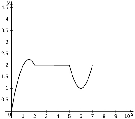
a. Use the graph of the position function to determine the time intervals when the velocity is positive, negative, or zero.

b. Sketch the graph of the velocity function.

c. Use the graph of the velocity function to determine the time intervals when the acceleration is positive, negative, or zero.

d. Determine the time intervals when the object is speeding up or slowing down.

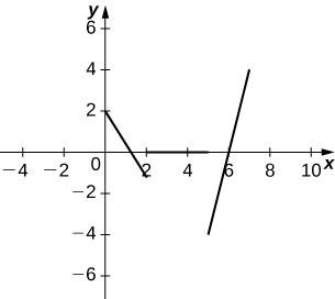
Solution: a. Velocity is positive on $(0,1.5)∪(6,7)$, negative on $(1.5,2)∪(5,6)$, and zero on $(2,5)$.

b.

c. Acceleration is positive on $(5,7)$, negative on $(0,2)$, and zero on $(2,5)$. d. The object is speeding up on $(6,7)∪(1.5,2)$ and slowing down on $(0,1.5)∪(5,6)$.

160) The cost function, in dollars, of a company that manufactures food processors is given by $C(x)=200+\frac{7}{x}+\frac{x}{27}$, where \(x\) is the number of food processors manufactured.

a. Find the marginal cost function.

b. Find the marginal cost of manufacturing 12 food processors.

c. Find the actual cost of manufacturing the thirteenth food processor.

161) The price p (in dollars) and the demand x for a certain digital clock radio is given by the price–demand function $p=10−0.001x$.

a. Find the revenue function $R(x)$

b. Find the marginal revenue function.

c. Find the marginal revenue at $x=2000$ and $5000$.

Solution: a. $R(x)=10x−0.001x^2$ b. $R′(x)=10−0.002x$ c. $6 per item, $0 per item

162) [T] A profit is earned when revenue exceeds cost. Suppose the profit function for a skateboard manufacturer is given by $P(x)=30x−0.3x^2−250$, where $x$ is the number of skateboards sold.

a. Find the exact profit from the sale of the thirtieth skateboard.

b. Find the marginal profit function and use it to estimate the profit from the sale of the thirtieth skateboard.

163) [T] In general, the profit function is the difference between the revenue and cost functions: $P(x)=R(x)−C(x)$.

Suppose the price-demand and cost functions for the production of cordless drills is given respectively by $p=143−0.03x$ and $C(x)=75,000+65x$, where $x$ is the number of cordless drills that are sold at a price of $p$ dollars per drill and $C(x)$ is the cost of producing $x$ cordless drills.

a. Find the marginal cost function.

b. Find the revenue and marginal revenue functions.

c. Find $R′(1000)$ and $R′(4000)$. Interpret the results.

d. Find the profit and marginal profit functions.

e. Find $P′(1000)$ and $P′(4000)$. Interpret the results.

Solution: a. $C′(x)=65$ b. $R(x)=143x−0.03x^2$, $R′(x)=143−0.06x$ c. $83,−97$. At a production level of 1000 cordless drills, revenue is increasing at a rate of $83 per drill; at a production level of 4000 cordless drills, revenue is decreasing at a rate of $97 per drill. d. $P(x)=−0.03x^2+78x−75000,P′(x)=−0.06x+78$ e. 18,−162. At a production level of 1000 cordless drills, profit is increasing at a rate of $18 per drill; at a production level of 4000 cordless drills, profit is decreasing at a rate of $162 per drill.

164) A small town in Ohio commissioned an actuarial firm to conduct a study that modeled the rate of change of the town’s population. The study found that the town’s population (measured in thousands of people) can be modeled by the function $P(t)=−\frac{1}{3}t^3+64t+3000$, where $t$ is measured in years.

a. Find the rate of change function $P′(t)$ of the population function.

b. Find $P′(1),P′(2),P′(3)$, and $P′(4)$. Interpret what the results mean for the town.

c. Find $P''(1),P''(2),P''(3)$, and $P''(4)$. Interpret what the results mean for the town’s population.

165) [T] A culture of bacteria grows in number according to the function $N(t)=3000(1+\frac{4t}{t^2+100})$, where $t$ is measured in hours.

a. Find the rate of change of the number of bacteria.

b. Find $N′(0),N′(10),N′(20)$, and $N′(30)$.

c. Interpret the results in (b).

d. Find $N''(0),N''(10),N''(20),$ and $N''(30)$. Interpret what the answers imply about the bacteria population growth.

Solution: a. $N′(t)=3000(\frac{−4t^2+400}{(t^2+100)}^2)$ b. $120,0,−14.4,−9.6$ c. The bacteria population increases from time 0 to 10 hours; afterwards, the bacteria population decreases. d. $0,−6,0.384,0.432$. The rate at which the bacteria is increasing is decreasing during the first 10 hours. Afterwards, the bacteria population is decreasing at a decreasing rate.

166) The centripetal force of an object of mass m is given by $F(r)=\frac{mv^2}{r}$, where $v$ is the speed of rotation and $r$ is the distance from the center of rotation.

a. Find the rate of change of centripetal force with respect to the distance from the center of rotation.

b. Find the rate of change of centripetal force of an object with mass 1000 kilograms, velocity of 13.89 m/s, and a distance from the center of rotation of 200 meters.

The following questions concern the population (in millions) of London by decade in the 19th century, which is listed in the following table.

Year Since 1800	Population (millions)
1	0.8975
11	1.040
21	1.264
31	1.516
41	1.661
51	2.000
61	2.634
71	3.272
81	3.911
91	4.422

Population of LondonSource: http://en.wikipedia.org/wiki/Demographics_of_London

167) [T]

a. Using a calculator or a computer program, find the best-fit linear function to measure the population.

b. Find the derivative of the equation in a. and explain its physical meaning.

c. Find the second derivative of the equation and explain its physical meaning.

Solution: a. $P(t)=0.03983+0.4280$ b. $P′(t)=0.03983$. The population is increasing. c. $P''(t)=0$. The rate at which the population is increasing is constant.

168) [T]

a. Using a calculator or a computer program, find the best-fit quadratic curve through the data.

b. Find the derivative of the equation and explain its physical meaning.

c. Find the second derivative of the equation and explain its physical meaning.