2.2E: Exercises for Section 2.2

Last updated
Save as PDF

Page ID: 48444

$ \newcommand{\vecs}[1]{\overset { \scriptstyle \rightharpoonup} {\mathbf{#1}} } $ $ \newcommand{\vecd}[1]{\overset{-\!-\!\rightharpoonup}{\vphantom{a}\smash {#1}}} $$\newcommand{\id}{\mathrm{id}}$ $ \newcommand{\Span}{\mathrm{span}}$ $ \newcommand{\kernel}{\mathrm{null}\,}$ $ \newcommand{\range}{\mathrm{range}\,}$ $ \newcommand{\RealPart}{\mathrm{Re}}$ $ \newcommand{\ImaginaryPart}{\mathrm{Im}}$ $ \newcommand{\Argument}{\mathrm{Arg}}$ $ \newcommand{\norm}[1]{\| #1 \|}$ $ \newcommand{\inner}[2]{\langle #1, #2 \rangle}$ $ \newcommand{\Span}{\mathrm{span}}$ $\newcommand{\id}{\mathrm{id}}$ $ \newcommand{\Span}{\mathrm{span}}$ $ \newcommand{\kernel}{\mathrm{null}\,}$ $ \newcommand{\range}{\mathrm{range}\,}$ $ \newcommand{\RealPart}{\mathrm{Re}}$ $ \newcommand{\ImaginaryPart}{\mathrm{Im}}$ $ \newcommand{\Argument}{\mathrm{Arg}}$ $ \newcommand{\norm}[1]{\| #1 \|}$ $ \newcommand{\inner}[2]{\langle #1, #2 \rangle}$ $ \newcommand{\Span}{\mathrm{span}}$$\newcommand{\AA}{\unicode[.8,0]{x212B}}$

Intuitive Definition of Limits

For exercises 1 - 2, consider the function $f(x)=\dfrac{x^2−1}{|x−1|}$.

1) [T] Complete the following table for the function. Round your solutions to four decimal places.

$x$	$f(x)$	$x$	$f(x)$
0.9	a.	1.1	e.
0.99	b.	1.01	f.
0.999	c.	1.001	g.
0.9999	d.	1.0001	h.

2) What do your results in the preceding exercise indicate about the two-sided limit $\displaystyle \lim_{x→1}f(x)$? Explain your response.

Answer:: $\displaystyle \lim_{x \to 1}f(x)$ does not exist because $\displaystyle \lim_{x \to 1^−}f(x)=−2≠\lim_{x \to 1^+}f(x)=2$.

For exercises 3 - 5, consider the function $f(x)=(1+x)^{1/x}$.

3) [T] Make a table showing the values of $f$ for $x=−0.01,\;−0.001,\;−0.0001,\;−0.00001$ and for $x=0.01,\;0.001,\;0.0001,\;0.00001$. Round your solutions to five decimal places.

$x$	$f(x)$	$x$	$f(x)$
-0.01	a.	0.01	e.
-0.001	b.	0.001	f.
-0.0001	c.	0.0001	g.
-0.00001	d.	0.00001	h.

4) What does the table of values in the preceding exercise indicate about the function $f(x)=(1+x)^{1/x}$?

Answer:: $\displaystyle \lim_{x \to 0}(1+x)^{1/x}\approx 2.7183$.

5) To which mathematical constant do the values in the preceding exercise appear to be approaching? This is the actual limit here.

In exercises 6 - 8, use the given values to set up a table to evaluate the limits. Round your solutions to eight decimal places.

6) [T] $\displaystyle \lim_{x \to 0}\frac{\sin 2x}{x};\quad ±0.1,\; ±0.01, \; ±0.001, \;±.0001$

$x$	$\frac{\sin 2x}{x}$	$x$	$\frac{\sin 2x}{x}$
-0.1	a.	0.1	e.
-0.01	b.	0.01	f.
-0.001	c.	0.001	g.
-0.0001	d.	0.0001	h.

Answer:: a. 1.98669331; b. 1.99986667; c. 1.99999867; d. 1.99999999; e. 1.98669331; f. 1.99986667; g. 1.99999867; h. 1.99999999;
$\displaystyle \lim_{x \to 0}\frac{\sin 2x}{x}=2$

7) [T] $\displaystyle \lim_{x \to 0}\frac{\sin 3x}{x} ±0.1, \; ±0.01, \; ±0.001, \; ±0.0001$

$x$	$\frac{\sin 3x}{x}$	$x$	$\frac{\sin 3x}{x}$
-0.1	a.	0.1	e.
-0.01	b.	0.01	f.
-0.001	c.	0.001	g.
-0.0001	d.	0.0001	h.

8) Use the preceding two exercises to conjecture (guess) the value of the following limit: $\displaystyle \lim_{x \to 0}\frac{\sin ax}{x}$ for $a$, a positive real value.

Answer:: $\displaystyle \lim_{x \to 0}\frac{\sin ax}{x}=a$

[T] In exercises 9 - 12, set up a table of values to find the indicated limit. Round to eight digits.

9) $\displaystyle \lim_{x \to 2}\frac{x^2−4}{x^2+x−6}$

$x$	$\frac{x^2−4}{x^2+x−6}$	$x$	$\frac{x^2−4}{x^2+x−6}$
1.9	a.	2.1	e.
1.99	b.	2.01	f.
1.999	c.	2.001	g.
1.9999	d.	2.0001	h.

10) $\displaystyle \lim_{x \to 1}(1−2x)$

$x$	$1−2x$	$x$	$1−2x$
0.9	a.	1.1	e.
0.99	b.	1.01	f.
0.999	c.	1.001	g.
0.9999	d.	1.0001	h.

Answer:: a. −0.80000000; b. −0.98000000; c. −0.99800000; d. −0.99980000; e. −1.2000000; f. −1.0200000; g. −1.0020000; h. −1.0002000;
$ \displaystyle \lim_{x \to 1}(1−2x)=−1$

11) $\displaystyle \lim_{x \to 0}\frac{5}{1−e^{1/x}}$

$x$	$\frac{5}{1−e^{1/x}}$	$x$	$\frac{5}{1−e^{1/x}}$
-0.1	a.	0.1	e.
-0.01	b.	0.01	f.
-0.001	c.	0.001	g.
-0.0001	d.	0.0001	h.

12) $\displaystyle \lim_{x \to 2}\frac{1−\frac{2}{x}}{x^2−4}$

$x$	$\frac{1−\frac{2}{x}}{x^2−4}$	$x$	$\frac{1−\frac{2}{x}}{x^2−4}$
1.9	a.	2.1	e.
1.99	b.	2.01	f.
1.999	c.	2.001	g.
1.9999	d.	2.0001	h.

Answer:: a. 0.13495277; b. 0.12594300; c. 0.12509381; d. 0.12500938; e. 0.11614402; f. 0.12406794; g. 0.12490631; h. 0.12499063;
$ \displaystyle ∴\lim_{x \to 2}\frac{1−\frac{2}{x}}{x^2−4}=0.1250=\frac{1}{8}$

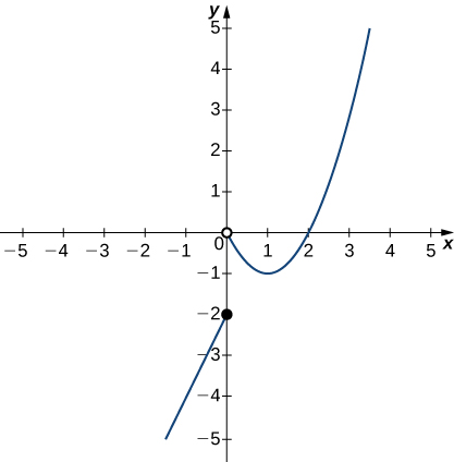
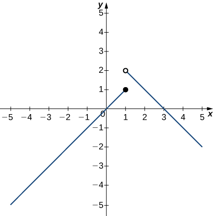
In exercises 13 - 17, use the following graph of the function $y=f(x)$ to find the values, if possible. Estimate when necessary.

$A graph of a piecewise function with two segments. The first segment exists for x <=1, and the second segment exists for x > 1. The first segment is linear with a slope of 1 and goes through the origin. Its endpoint is a closed circle at (1,1). The second segment is also linear with a slope of -1. It begins with the open circle at (1,2).$

13) $\displaystyle \lim_{x→1^−}f(x)$

14) $\displaystyle \lim_{x→1^+}f(x)$

Answer:: $2$

15) $\displaystyle \lim_{x→1}f(x)$

16) $\displaystyle \lim_{x→2}f(x)$

Answer:: $1$

17) $f(1)$

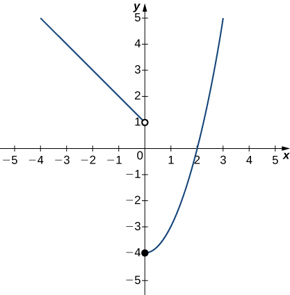
In exercises 18 - 21, use the graph of the function $y=f(x)$ shown here to find the values, if possible. Estimate when necessary.

$A graph of a piecewise function with two segments. The first is a linear function for x < 0. There is an open circle at (0,1), and its slope is -1. The second segment is the right half of a parabola opening upward. Its vertex is a closed circle at (0, -4), and it goes through the point (2,0).$

18) $\displaystyle \lim_{x→0^−}f(x)$

Answer:: $1$

19) $\displaystyle \lim_{x→0^+}f(x)$

20) $\displaystyle \lim_{x→0}f(x)$

Answer:: DNE

21) $\displaystyle \lim_{x→2}f(x)$

In exercises 22 - 27, use the graph of the function $y=f(x)$ shown here to find the values, if possible. Estimate when necessary.

$A graph of a piecewise function with three segments, all linear. The first exists for x < -2, has a slope of 1, and ends at the open circle at (-2, 0). The second exists over the interval [-2, 2], has a slope of -1, goes through the origin, and has closed circles at its endpoints (-2, 2) and (2,-2). The third exists for x>2, has a slope of 1, and begins at the open circle (2,2).$

22) $\displaystyle \lim_{x→−2^−}f(x)$

Answer:: $0$

23) $\displaystyle \lim_{x→−2^+}f(x)$

24) $\displaystyle \lim_{x→−2}f(x)$

Answer:: DNE

25) $\displaystyle \lim_{x→2^−}f(x)$

26) $\displaystyle \lim_{x→2^+}f(x)$

Answer:: $2$

27) $\displaystyle \lim_{x→2}f(x)$

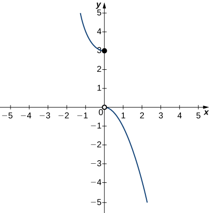
In exercises 28 - 30, use the graph of the function $y=g(x)$ shown here to find the values, if possible. Estimate when necessary.

$A graph of a piecewise function with two segments. The first exists for x>=0 and is the left half of an upward opening parabola with vertex at the closed circle (0,3). The second exists for x>0 and is the right half of a downward opening parabola with vertex at the open circle (0,0).$

28) $\displaystyle \lim_{x→0^−}g(x)$

Answer:: $3$

29) $\displaystyle \lim_{x→0^+}g(x)$

30) $\displaystyle \lim_{x→0}g(x)$

Answer:: DNE

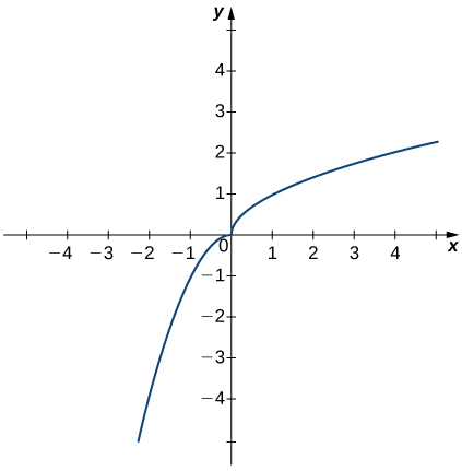
In exercises 31 - 33, use the graph of the function $y=h(x)$ shown here to find the values, if possible. Estimate when necessary.

$A graph of a function with two curves approaching 0 from quadrant 1 and quadrant 3. The curve in quadrant one appears to be the top half of a parabola opening to the right of the y axis along the x axis with vertex at the origin. The curve in quadrant three appears to be the left half of a parabola opening downward with vertex at the origin.$

31) $\displaystyle \lim_{x→0^−}h(x)$

32) $\displaystyle \lim_{x→0^+}h(x)$

Answer:: $0$

33) $\displaystyle \lim_{x→0}h(x)$

In exercises 34 - 38, use the graph of the function $y=f(x)$ shown here to find the values, if possible. Estimate when necessary.

$A graph with a curve and a point. The point is a closed circle at (0,-2). The curve is part of an upward opening parabola with vertex at (1,-1). It exists for x > 0, and there is a closed circle at the origin.$

34) $\displaystyle \lim_{x→0^−}f(x)$

Answer:: $-2$

35) $\displaystyle \lim_{x→0^+}f(x)$

36) $\displaystyle \lim_{x→0}f(x)$

Answer:: DNE

37) $\displaystyle \lim_{x→1}f(x)$

38) $\displaystyle \lim_{x→2}f(x)$

Answer:: $0$

39) A track coach uses a camera with a fast shutter to estimate the position of a runner with respect to time. A table of the values of position of the athlete versus time is given here, where $x$ is the position in meters of the runner and $t$ is time in seconds. What is $\displaystyle \lim_{t→2}\;x(t)$? What does it mean physically?

$t(sec)$	$x(m)$
1.75	4.5
1.95	6.1
1.99	6.42
2.01	6.58
2.05	6.9
2.25	8.5

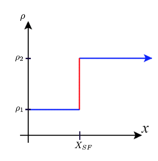
40) Shock waves arise in many physical applications, ranging from supernovas to detonation waves. A graph of the density of a shock wave with respect to distance, $x$, is shown here. We are mainly interested in the location of the front of the shock, labeled $X_{SF}$ in the diagram.

$A graph in quadrant one of the density of a shockwave with three labeled points: p1 and p2 on the y axis, with p1 > p2, and xsf on the x axis. It consists of y= p1 from 0 to xsf, x = xsf from y= p1 to y=p2, and y=p2 for values greater than or equal to xsf.$

a. Evaluate $\displaystyle \lim_{x→X_{SF}^+}ρ(x)$.

b. Evaluate $\displaystyle \lim_{x→X_{SF}^−}ρ(x)$.

c. Evaluate $\displaystyle \lim_{x→X_{SF}}ρ(x)$. Explain the physical meanings behind your answers.

Answer:: a. $ρ_2$ b. $ρ_1$ c. DNE unless $ρ_1=ρ_2$. As you approach $X_{SF}$ from the right, you are in the high-density area of the shock. When you approach from the left, you have not experienced the “shock” yet and are at a lower density.

Contributors and Attributions

Gilbert Strang (MIT) and Edwin “Jed” Herman (Harvey Mudd) with many contributing authors. This content by OpenStax is licensed with a CC-BY-SA-NC 4.0 license. Download for free at http://cnx.org.