2.3E: Exercises for Section 2.3

Last updated
Save as PDF

Page ID: 48929

$ \newcommand{\vecs}[1]{\overset { \scriptstyle \rightharpoonup} {\mathbf{#1}} } $

$ \newcommand{\vecd}[1]{\overset{-\!-\!\rightharpoonup}{\vphantom{a}\smash {#1}}} $

$ \newcommand{\id}{\mathrm{id}}$ $ \newcommand{\Span}{\mathrm{span}}$

( \newcommand{\kernel}{\mathrm{null}\,}\) $ \newcommand{\range}{\mathrm{range}\,}$

$ \newcommand{\RealPart}{\mathrm{Re}}$ $ \newcommand{\ImaginaryPart}{\mathrm{Im}}$

$ \newcommand{\Argument}{\mathrm{Arg}}$ $ \newcommand{\norm}[1]{\| #1 \|}$

$ \newcommand{\inner}[2]{\langle #1, #2 \rangle}$

$ \newcommand{\Span}{\mathrm{span}}$

$ \newcommand{\id}{\mathrm{id}}$

$ \newcommand{\Span}{\mathrm{span}}$

$ \newcommand{\kernel}{\mathrm{null}\,}$

$ \newcommand{\range}{\mathrm{range}\,}$

$ \newcommand{\RealPart}{\mathrm{Re}}$

$ \newcommand{\ImaginaryPart}{\mathrm{Im}}$

$ \newcommand{\Argument}{\mathrm{Arg}}$

$ \newcommand{\norm}[1]{\| #1 \|}$

$ \newcommand{\inner}[2]{\langle #1, #2 \rangle}$

$ \newcommand{\Span}{\mathrm{span}}$ $ \newcommand{\AA}{\unicode[.8,0]{x212B}}$

$ \newcommand{\vectorA}[1]{\vec{#1}} % arrow$

$ \newcommand{\vectorAt}[1]{\vec{\text{#1}}} % arrow$

$ \newcommand{\vectorB}[1]{\overset { \scriptstyle \rightharpoonup} {\mathbf{#1}} } $

$ \newcommand{\vectorC}[1]{\textbf{#1}} $

$ \newcommand{\vectorD}[1]{\overrightarrow{#1}} $

$ \newcommand{\vectorDt}[1]{\overrightarrow{\text{#1}}} $

$ \newcommand{\vectE}[1]{\overset{-\!-\!\rightharpoonup}{\vphantom{a}\smash{\mathbf {#1}}}} $

$ \newcommand{\vecs}[1]{\overset { \scriptstyle \rightharpoonup} {\mathbf{#1}} } $

$ \newcommand{\vecd}[1]{\overset{-\!-\!\rightharpoonup}{\vphantom{a}\smash {#1}}} $

$\newcommand{\avec}{\mathbf a}$ $\newcommand{\bvec}{\mathbf b}$ $\newcommand{\cvec}{\mathbf c}$ $\newcommand{\dvec}{\mathbf d}$ $\newcommand{\dtil}{\widetilde{\mathbf d}}$ $\newcommand{\evec}{\mathbf e}$ $\newcommand{\fvec}{\mathbf f}$ $\newcommand{\nvec}{\mathbf n}$ $\newcommand{\pvec}{\mathbf p}$ $\newcommand{\qvec}{\mathbf q}$ $\newcommand{\svec}{\mathbf s}$ $\newcommand{\tvec}{\mathbf t}$ $\newcommand{\uvec}{\mathbf u}$ $\newcommand{\vvec}{\mathbf v}$ $\newcommand{\wvec}{\mathbf w}$ $\newcommand{\xvec}{\mathbf x}$ $\newcommand{\yvec}{\mathbf y}$ $\newcommand{\zvec}{\mathbf z}$ $\newcommand{\rvec}{\mathbf r}$ $\newcommand{\mvec}{\mathbf m}$ $\newcommand{\zerovec}{\mathbf 0}$ $\newcommand{\onevec}{\mathbf 1}$ $\newcommand{\real}{\mathbb R}$ $\newcommand{\twovec}[2]{\left[\begin{array}{r}#1 \\ #2 \end{array}\right]}$ $\newcommand{\ctwovec}[2]{\left[\begin{array}{c}#1 \\ #2 \end{array}\right]}$ $\newcommand{\threevec}[3]{\left[\begin{array}{r}#1 \\ #2 \\ #3 \end{array}\right]}$ $\newcommand{\cthreevec}[3]{\left[\begin{array}{c}#1 \\ #2 \\ #3 \end{array}\right]}$ $\newcommand{\fourvec}[4]{\left[\begin{array}{r}#1 \\ #2 \\ #3 \\ #4 \end{array}\right]}$ $\newcommand{\cfourvec}[4]{\left[\begin{array}{c}#1 \\ #2 \\ #3 \\ #4 \end{array}\right]}$ $\newcommand{\fivevec}[5]{\left[\begin{array}{r}#1 \\ #2 \\ #3 \\ #4 \\ #5 \\ \end{array}\right]}$ $\newcommand{\cfivevec}[5]{\left[\begin{array}{c}#1 \\ #2 \\ #3 \\ #4 \\ #5 \\ \end{array}\right]}$ $\newcommand{\mattwo}[4]{\left[\begin{array}{rr}#1 \amp #2 \\ #3 \amp #4 \\ \end{array}\right]}$ $\newcommand{\laspan}[1]{\text{Span}\{#1\}}$ $\newcommand{\bcal}{\cal B}$ $\newcommand{\ccal}{\cal C}$ $\newcommand{\scal}{\cal S}$ $\newcommand{\wcal}{\cal W}$ $\newcommand{\ecal}{\cal E}$ $\newcommand{\coords}[2]{\left\{#1\right\}_{#2}}$ $\newcommand{\gray}[1]{\color{gray}{#1}}$ $\newcommand{\lgray}[1]{\color{lightgray}{#1}}$ $\newcommand{\rank}{\operatorname{rank}}$ $\newcommand{\row}{\text{Row}}$ $\newcommand{\col}{\text{Col}}$ $\renewcommand{\row}{\text{Row}}$ $\newcommand{\nul}{\text{Nul}}$ $\newcommand{\var}{\text{Var}}$ $\newcommand{\corr}{\text{corr}}$ $\newcommand{\len}[1]{\left|#1\right|}$ $\newcommand{\bbar}{\overline{\bvec}}$ $\newcommand{\bhat}{\widehat{\bvec}}$ $\newcommand{\bperp}{\bvec^\perp}$ $\newcommand{\xhat}{\widehat{\xvec}}$ $\newcommand{\vhat}{\widehat{\vvec}}$ $\newcommand{\uhat}{\widehat{\uvec}}$ $\newcommand{\what}{\widehat{\wvec}}$ $\newcommand{\Sighat}{\widehat{\Sigma}}$ $\newcommand{\lt}{<}$ $\newcommand{\gt}{>}$ $\newcommand{\amp}{&}$ $\definecolor{fillinmathshade}{gray}{0.9}$

Infinite Limits

[T] In exercises 1 - 2, set up a table of values to find the indicated limit. Round to eight significant digits.

1) $\displaystyle \lim_{z \to 0}\frac{z−1}{z^2(z+3)}$

$z$	$\frac{z−1}{z^2(z+3)}$	$z$	$\frac{z−1}{z^2(z+3)}$
-0.1	a.	0.1	e.
-0.01	b.	0.01	f.
-0.001	c.	0.001	g.
-0.0001	d.	0.0001	h.

Answer:: a. −37.931034; b. −3377.9264; c. −333,777.93; d. −33,337,778; e. −29.032258; f. −3289.0365; g. −332,889.04; h. −33,328,889
$ \displaystyle \lim_{x \to 0}\frac{z−1}{z^2(z+3)}=−∞$

2) $\displaystyle \lim_{t \to 0^+}\frac{\cos t}{t}$

$t$	$\frac{\cos t}{t}$
0.1	a.
0.01	b.
0.001	c.
0.0001	d.

[T] In exercises 3 - 4, set up a table of values and round to eight significant digits. Based on the table of values, make a guess about what the limit is. Then, use a calculator to graph the function and determine the limit. Was the conjecture correct? If not, why does the method of tables fail?

3) $\displaystyle \lim_{α \to 0^+} \frac{1}{α}\cos\left(\frac{π}{α}\right)$

$a$	$\frac{1}{α}\cos\left(\frac{π}{α}\right)$
0.1	a.
0.01	b.
0.001	c.
0.0001	d.

Answer:

a. 10.00000; b. 100.00000; c. 1000.0000; d. 10,000.000;
Guess: $\displaystyle \lim_{α→0^+}\frac{1}{α}\cos\left(\frac{π}{α}\right)=∞$;
Actual: DNE, since the graph shows the function oscillates wildly between values approaching positive infinity and values approaching negative infinity, as the value of $α$ approaches $0$ from the positive side.

$A graph of the function (1/alpha) * cos (pi / alpha), which oscillates gently until the interval [-.2, .2], where it oscillates rapidly, going to infinity and negative infinity as it approaches the y axis.$

4) $\displaystyle \lim_{θ \to 0}\sin\left(\frac{π}{θ}\right)$

$θ$	$\sin\left(\frac{π}{θ}\right)$	$θ$	$\sin\left(\frac{π}{θ}\right)$
-0.1	a.	0.1	e.
-0.01	b.	0.01	f.
-0.001	c.	0.001	g.
-0.0001	d.	0.0001	h.

In exercises 5 - 8, consider the graph of the function $y=f(x)$ shown here. Which of the statements about $y=f(x)$ are true and which are false? Explain why a statement is false.

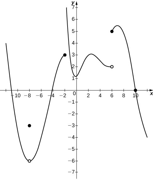
$A graph of a piecewise function with three segments and a point. The first segment is a curve opening upward with vertex at (-8, -6). This vertex is an open circle, and there is a closed circle instead at (-8, -3). The segment ends at (-2,3), where there is a closed circle. The second segment stretches up asymptotically to infinity along x=-2, changes direction to increasing at about (0,1.25), increases until about (2.25, 3), and decreases until (6,2), where there is an open circle. The last segment starts at (6,5), increases slightly, and then decreases into quadrant four, crossing the x axis at (10,0). All of the changes in direction are smooth curves.$

5) $\displaystyle \lim_{x→−2^+}f(x)=3$

Answer:: False; $\displaystyle \lim_{x→−2^+}f(x)=+∞$

6) $\displaystyle \lim_{x→−8}f(x)=f(−8)$

7) $\displaystyle \lim_{x→6}f(x)=5$

Answer:: False; $\displaystyle \lim_{x→6}f(x)$ DNE since $\displaystyle \lim_{x→6^−}f(x)=2$ and $\displaystyle \lim_{x→6^+}f(x)=5$.

8) $\displaystyle \lim_{x→10}f(x)=0$

In each exercise, sketch the graph of a function with the given properties.

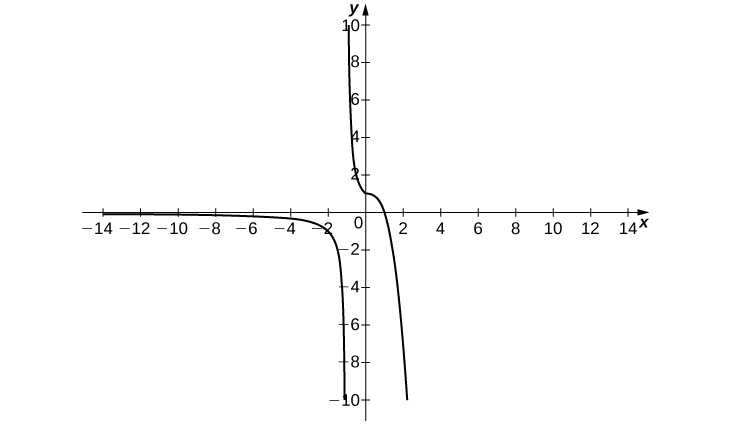
9) $\displaystyle \lim_{x→−∞}f(x)=0, \quad \lim_{x→−1^−}f(x)=−∞, \quad \lim_{x→−1^+}f(x)=∞,\quad \lim_{x→0}f(x)=f(0), \quad f(0)=1, \quad \lim_{x→∞}f(x)=−∞$

Answer:

Answers may vary

$A graph of a piecewise function with two segments. The first segment is in quadrant three and asymptotically goes to negative infinity along the y axis and 0 along the x axis. The second segment consists of two curves. The first appears to be the left half of an upward opening parabola with vertex at (0,1). The second appears to be the right half of a downward opening parabola with vertex at (0,1) as well.$

10) $\displaystyle \lim_{x→2}f(x)=1, \quad \lim_{x→4^−}f(x)=3, \quad \lim_{x→4^+}f(x)=6, \quad x=4$ is not defined.

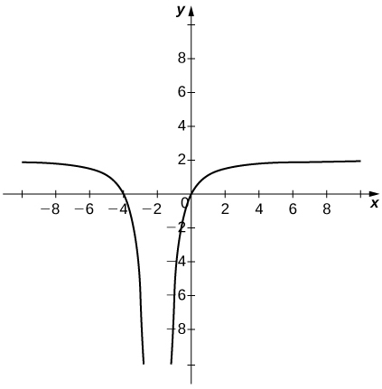
11) $\displaystyle \lim_{x→−∞}f(x)=2,\quad \lim_{x→−2}f(x)=−∞,\quad \lim_{x→∞}f(x)=2,\quad f(0)=0$

Answer:

Answer may vary

$A graph containing two curves. The first goes to 2 asymptotically along y=2 and to negative infinity along x = -2. The second goes to negative infinity along x=-2 and to 2 along y=2.$

12) $\displaystyle \lim_{x→−∞}f(x)=2, \quad \lim_{x→3^−}f(x)=−∞, \quad \lim_{x→3^+}f(x)=∞, \quad \lim_{x→∞}f(x)=2, \quad f(0)=-\frac{1}{3}$

13) $\displaystyle \lim_{x→−∞}f(x)=0,\quad \lim_{x→−1^−}f(x)=∞,\quad \lim_{x→−1^+}f(x)=−∞, \quad f(0)=−1, \quad \lim_{x→1^−}f(x)=−∞, \quad \lim_{x→1^+}f(x)=∞, \quad \lim_{x→∞}f(x)=0$

Contributors and Attributions

Gilbert Strang (MIT) and Edwin “Jed” Herman (Harvey Mudd) with many contributing authors. This content by OpenStax is licensed with a CC-BY-SA-NC 4.0 license. Download for free at http://cnx.org.

Search

Text Color

Text Size

Margin Size

Font Type