4.8: Derivatives of Parametric Equations

Learning Objectives

• Determine the first and second derivatives of parametric equations
• Determine the equations of tangent lines to parametric curves.
• Find the speed at any point in time for motion along a given parametric curve.

Now that we have introduced the concept of a parameterized curve, our next step is to learn how to work with this concept in the context of calculus. For example, if we know a parameterization of a given curve, how can we calculate the slope of a tangent line to the curve?

Another scenario: Suppose we would like to represent the location of a baseball after the ball leaves a pitcher’s hand. If the position of the baseball is represented by the plane curve \((x(t),y(t))\) then we should be able to use calculus to find the speed of the ball at any given time.

Derivatives of Parametric Equations

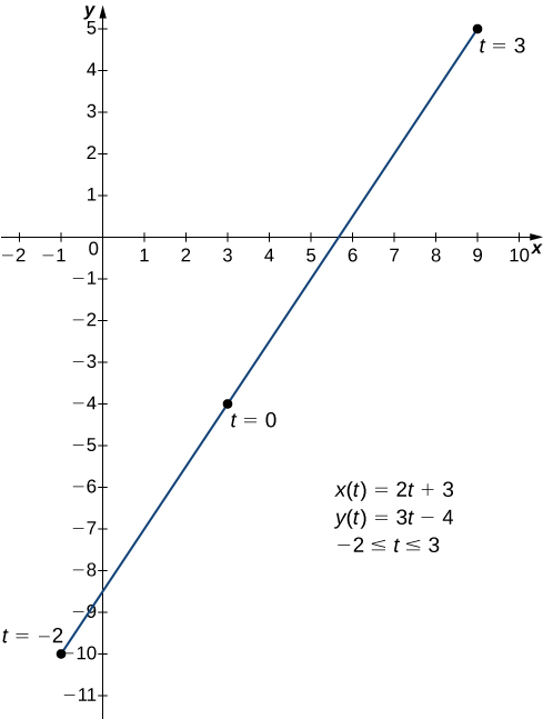
We start by asking how to calculate the slope of a line tangent to a parametric curve at a point. Consider the plane curve defined by the parametric equations

\[\begin{align} x(t) &=2t+3 \label{eq1} \\ y(t) &=3t−4 \label{eq2} \end{align} \]

within \(−2≤t≤3\).

The graph of this curve appears in Figure \(\PageIndex{1}\). It is a line segment starting at \((−1,−10)\) and ending at \((9,5).\)

Figure \(\PageIndex{1}\): Graph of the line segment described by the given parametric equations.

We can eliminate the parameter by first solving Equation \ref{eq1} for \(t\):

\(x(t)=2t+3\)

\(x−3=2t\)

\(t=\dfrac{x−3}{2}\).

Substituting this into \(y(t)\) (Equation \ref{eq2}), we obtain

\(y(t)=3t−4\)

\(y=3\left(\dfrac{x−3}{2}\right)−4\)

\(y=\dfrac{3x}{2}−\dfrac{9}{2}−4\)

\(y=\dfrac{3x}{2}−\dfrac{17}{2}\).

The slope of this line is given by \(\dfrac{dy}{dx}=\dfrac{3}{2}\). Next we calculate \(x′(t)\) and \(y′(t)\). This gives \(x′(t)=2\) and \(y′(t)=3\). Notice that

\[\dfrac{dy}{dx}=\dfrac{dy/dt}{dx/dt}=\dfrac{3}{2}. \nonumber \]

This is no coincidence, as outlined in the following theorem.

Derivative of Parametric Equations

Consider the plane curve defined by the parametric equations \(x=x(t)\) and \(y=y(t)\). Suppose that \(x′(t)\) and \(y′(t)\) exist, and assume that \(x′(t)≠0\). Then the derivative \(\dfrac{dy}{dx}\)is given by

\[\dfrac{dy}{dx}=\dfrac{dy/dt}{dx/dt}=\dfrac{y′(t)}{x′(t)}. \label{paraD} \]

Proof

This theorem can be proven using the Chain Rule. In particular, assume that the parameter \(t\) can be eliminated, yielding a differentiable function \(y=F(x)\). Then \(y(t)=F(x(t)).\) Differentiating both sides of this equation using the Chain Rule yields

\[y′(t)=F′\big(x(t)\big)x′(t), \nonumber \]

so

\[F′\big(x(t)\big)=\dfrac{y′(t)}{x′(t)}. \nonumber \]

But \(F′\big(x(t)\big)=\dfrac{dy}{dx}\), which proves the theorem.

□

Equation \ref{paraD} can be used to calculate derivatives of plane curves, as well as critical points. Recall that a critical point of a differentiable function \(y=f(x)\) is any point \(x=x_0\) such that either \(f′(x_0)=0\) or \(f′(x_0)\) does not exist. Equation \ref{paraD} gives a formula for the slope of a tangent line to a curve defined parametrically regardless of whether the curve can be described by a function \(y=f(x)\) or not.

Example \(\PageIndex{1}\): Finding the Derivative of a Parametric Curve

Calculate the derivative \(\dfrac{dy}{dx}\) for each of the following parametrically defined plane curves, and locate any critical points on their respective graphs.

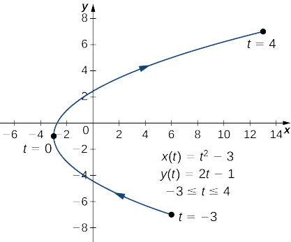
1. \(x(t)=t^2−3, \quad y(t)=2t−1, \quad\text{for }−3≤t≤4\)
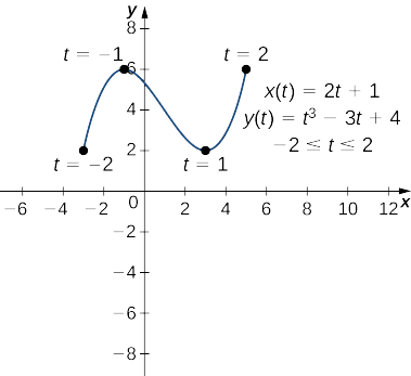
2. \(x(t)=2t+1, \quad y(t)=t^3−3t+4, \quad\text{for }−2≤t≤2\)
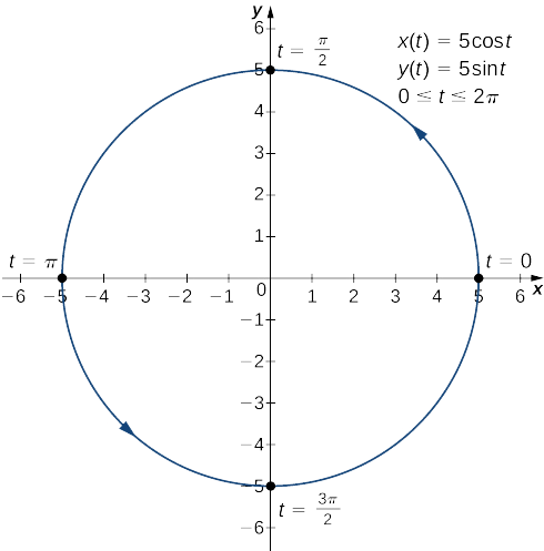
3. \(x(t)=5\cos t, \quad y(t)=5\sin t, \quad\text{for }0≤t≤2π\)

Solution

a. To apply Equation \ref{paraD}, first calculate \(x′(t)\) and \(y′(t)\):

\(x′(t)=2t\)

\(y′(t)=2\).

Next substitute these into the equation:

\(\dfrac{dy}{dx}=\dfrac{dy/dt}{dx/dt}\)

\(\dfrac{dy}{dx}=\dfrac{2}{2t}\)

\(\dfrac{dy}{dx}=\dfrac{1}{t}\).

This derivative is undefined when \(t=0\). Calculating \(x(0)\) and \(y(0)\) gives \(x(0)=(0)^2−3=−3\) and \(y(0)=2(0)−1=−1\), which corresponds to the point \((−3,−1)\) on the graph. The graph of this curve is a parabola opening to the right, and the point \((−3,−1)\) is its vertex as shown.

Figure \(\PageIndex{2}\): Graph of the parabola described by parametric equations in part a.

b. To apply Equation \ref{paraD}, first calculate \(x′(t)\) and \(y′(t)\):

\(x′(t)=2\)

\(y′(t)=3t^2−3\).

Next substitute these into the equation:

\(\dfrac{dy}{dx}=\dfrac{dy/dt}{dx/dt}\)

\(\dfrac{dy}{dx}=\dfrac{3t^2−3}{2}\).

This derivative is zero when \(t=±1\). When \(t=−1\) we have

\(x(−1)=2(−1)+1=−1\) and \(y(−1)=(−1)^3−3(−1)+4=−1+3+4=6\),

which corresponds to the point \((−1,6)\) on the graph. When \(t=1\) we have

\(x(1)=2(1)+1=3\) and \(y(1)=(1)^3−3(1)+4=1−3+4=2,\)

which corresponds to the point \((3,2)\) on the graph. The point \((3,2)\) is a relative minimum and the point \((−1,6)\) is a relative maximum, as seen in the following graph.

Figure \(\PageIndex{3}\): Graph of the curve described by parametric equations in part b.

c. To apply Equation \ref{paraD}, first calculate \(x′(t)\) and \(y′(t)\):

\(x′(t)=−5\sin t\)

\(y′(t)=5\cos t.\)

Next substitute these into the equation:

\(\dfrac{dy}{dx}=\dfrac{dy/dt}{dx/dt}\)

\(\dfrac{dy}{dx}=\dfrac{5\cos t}{−5\sin t}\)

\(\dfrac{dy}{dx}=−\cot t.\)

This derivative is zero when \(\cos t=0\) and is undefined when \(\sin t=0.\) This gives \(t=0,\dfrac{π}{2},π,\dfrac{3π}{2},\) and \(2π\) as critical points for t. Substituting each of these into \(x(t)\) and \(y(t)\), we obtain

\(t\)	\(x(t)\)	\(y(t)\)
0	5	0
\(\dfrac{π}{2}\)	0	5
\(π\)	−5	0
\(\dfrac{3π}{2}\)	0	−5
\(2π\)	5	0

These points correspond to the sides, top, and bottom of the circle that is represented by the parametric equations (Figure \(\PageIndex{4}\)). On the left and right edges of the circle, the derivative is undefined, and on the top and bottom, the derivative equals zero.

Figure \(\PageIndex{4}\): Graph of the curve described by parametric equations in part c.

Exercise \(\PageIndex{1}\)

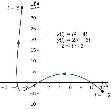
Calculate the derivative \(dy/dx\) for the plane curve defined by the equations

\[x(t)=t^2−4t, \quad y(t)=2t^3−6t, \quad\text{for }−2≤t≤3 \nonumber \]

and locate any critical points on its graph.

Hint

Calculate \(x′(t)\) and \(y′(t)\) and use Equation \ref{paraD}.

Answer

\(x′(t)=2t−4\) and \(y′(t)=6t^2−6\), so \(\dfrac{dy}{dx}=\dfrac{6t^2−6}{2t−4}=\dfrac{3t^2−3}{t−2}\).

This expression is undefined when \(t=2\) and equal to zero when \(t=±1\).

Example \(\PageIndex{2}\): Finding a Tangent Line

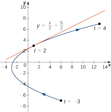
Find the equation of the tangent line to the curve defined by the equations

\[x(t)=t^2−3, \quad y(t)=2t−1, \quad\text{for }−3≤t≤4 \nonumber \]

when \(t=2\).

Solution

First find the slope of the tangent line using Equation \ref{paraD}, which means calculating \(x′(t)\) and \(y′(t)\):

\(x′(t)=2t\)

\(y′(t)=2\).

Next substitute these into the equation:

\(\dfrac{dy}{dx}=\dfrac{dy/dt}{dx/dt}\)

\(\dfrac{dy}{dx}=\dfrac{2}{2t}\)

\(\dfrac{dy}{dx}=\dfrac{1}{t}\).

When \(t=2, \dfrac{dy}{dx}=\dfrac{1}{2}\), so this is the slope of the tangent line. Calculating \(x(2)\) and \(y(2)\) gives

\(x(2)=(2)^2−3=1\) and \(y(2)=2(2)−1=3\),

which corresponds to the point \((1,3)\) on the graph (Figure \(\PageIndex{5}\)). Now use the point-slope form of the equation of a line to find the equation of the tangent line:

\(y−y_0=m(x−x_0)\)

\(y−3=\dfrac{1}{2}(x−1)\)

\(y−3=\dfrac{1}{2}x−\dfrac{1}{2}\)

\(y=\dfrac{1}{2}x+\dfrac{5}{2}\).

Figure \(\PageIndex{5}\): Tangent line to the parabola described by the given parametric equations when \(t=2\).

Exercise \(\PageIndex{2}\)

Find the equation of the tangent line to the curve defined by the equations

\(x(t)=t^2−4t, \quad y(t)=2t^3−6t, \quad\text{for }−2≤t≤6\) when \(t=5\).

Hint

Calculate \(x′(t)\) and \(y′(t)\) and use Equation \ref{paraD}.

Answer

The equation of the tangent line is \(y=24x+100.\)

Second-Order Derivatives

Our next goal is to see how to take the second derivative of a function defined parametrically. The second derivative of a function \(y=f(x)\) is defined to be the derivative of the first derivative; that is,

\[\dfrac{d^2y}{dx^2}=\dfrac{d}{dx}\left[\dfrac{dy}{dx}\right]. \label{eqD2} \]

Since

\[\dfrac{dy}{dx}=\dfrac{dy/dt}{dx/dt}, \nonumber \]

we can replace the \(y\) on both sides of Equation \ref{eqD2} with \(\dfrac{dy}{dx}\). This gives us

\[\dfrac{d^2y}{dx^2}=\dfrac{d}{dx} \left(\dfrac{dy}{dx} \right)=\dfrac{(d/dt)(dy/dx)}{dx/dt}.\label{paraD2} \]

If we know \(dy/dx\) as a function of \(t\), then this formula is straightforward to apply

Example \(\PageIndex{3}\): Finding a Second Derivative

Calculate the second derivative \(d^2y/dx^2\) for the plane curve defined by the parametric equations \(x(t)=t^2−3, \quad y(t)=2t−1, \quad\text{for }−3≤t≤4.\)

Solution

From Example \(\PageIndex{1}\) we know that \(\dfrac{dy}{dx}=\dfrac{2}{2t}=\dfrac{1}{t}\). Using Equation \ref{paraD2}, we obtain

\(\dfrac{d^2y}{dx^2}=\dfrac{(d/dt)(dy/dx)}{dx/dt}=\dfrac{(d/dt)(1/t)}{2t}=\dfrac{−t^{−2}}{2t}=−\dfrac{1}{2t^3}\).

Exercise \(\PageIndex{3}\)

Calculate the second derivative \(d^2y/dx^2\) for the plane curve defined by the equations

\(x(t)=t^2−4t, \quad y(t)=2t^3−6t, \quad\text{for }−2≤t≤3\)

and locate any critical points on its graph.

Hint

Start with the solution from the previous exercise, and use Equation \ref{paraD2}.

Answer

\(\dfrac{d^2y}{dx^2}=\dfrac{3t^2−12t+3}{2(t−2)^3}\). Critical points \((5,4),\, (−3,−4)\),and \((−4,6).\)

Speed along a Parametric Curve

As we discussed earlier in this course, where we considered rectilinear motion (motion along a straight line), the velocity of a particle is the derivative of the position function describing the particle's motion.  Since a set of parametric equations together describe the position of an object along a curve, the derivative of these parametric equations together describe the velocity of this object at any given time along its parameterized path.

So, for example, if an object's motion is described by the parametric equations,

\[\begin{align*} x(t) &= t \\ y(t) &= t^2, \end{align*}\]

then the velocity of this object's motion is described by the parametric equations,

\[\begin{align*} x'(t) &= 1 \\ y'(t) &= 2t. \end{align*}\]

Now, remember that speed is the the magnitude of the velocity.  So, in rectilinear motion, it is found by taking the absolute value of the signed velocity.  This ignores the direction of the motion implied by the positive or negative sign of the velocity in this case.

But for parametric curves, the velocity is actually a vector that not only incorporates the speed of the motion, but also the direction of the motion (tangent to the curve) at any given point.

So in the example above, at time \(t = 1\), the position of the object would be given by \(\Big(x(1), y(1)\Big) = (1, 1)\).  The velocity at this point, given by \(x'(t) = 1\) and \(y'(t) = 2t\), is in the direction given by evaluating these functions at \(t=1\), i.e., since \(x'(1) = 1\) and \(y'(1) = 2\), we know that at the point \((1, 1)\), the velocity is in the direction \(1\) unit to the right and \(2\) units up.  If we draw this vector (a segment with an arrow to indicate the direction), we can intuitively determine the speed by calculating the magnitude (length) of this segment.

Thus, using the distance formula (or just the Pythagorean Theorem on which it is based), we find that the speed here is given by:

\[\text{Speed}(1) =\sqrt{\big(x'(1)\big)^2 + \big(y'(1)\big)^2 } = \sqrt{1^2 + 2^2} = \sqrt{5}\nonumber\]

If distance were measured here in feet and time in seconds, then the speed of the object at time \(t = 1\) seconds would be \(\sqrt{5}\) ft/sec.

We can generalize this result to state a formula for the speed of an object's motion along any given parametric curve.

Definition: Speed and Direction of Motion along a Parametric Curve

If the motion of an object are given by the parametric equations, \(x(t)\) an \(y(t)\), then the speed of the object along the path given by the parametric equations at any time \(t\) will be given by the formula:

\[\text{Speed}(t) = \sqrt{\big(x'(t)\big)^2 + \big(y'(t)\big)^2}.\]

The direction of the motion along the curve at any time \(t\) is given by the signed values of the derivatives \(x'(t)\) and \(y'(t)\), and will be along the line tangent to the parametric curve at this point.

Let's look at an example where we find the speed of the motion along a parametric curve as a function of time \(t\).

Example \(\PageIndex{4a}\)

Find the speed of the motion along the following parameterized curve as a function of time \(t\).

\[\begin{align*} x(t) &= t \\ y(t) &= t^2, \end{align*}\]

Figure \(\PageIndex{6}\): Graph of this parametric curve

Solution

Since the speed in the \(x\)-direction is given by \(x'(t) = 1\) and the speed in the \(y\)-direction is given by \(y'(t) = 2t\), we have,

\[\text{Speed}(t) = \sqrt{(1)^2 + (2t)^2} =\sqrt{1 + 4t^2}.\nonumber\]

Note that in Example \(\PageIndex{4}\) we can see that the speed varies as time passes.  Is there a relative maximum speed or relative minimum speed for any value(s) of \(t\)?

Using what we learned earlier, we can check this function for critical numbers and determine whether it has any relative extrema.

We can take advantage of a useful fact when looking for relative extrema in speed functions.

Normally, a square root function can have critical numbers (and relative extrema) at values of the independent variable where the derivative does not exist and there is a cusp in its graph, i.e., where the original function crosses the \(x\)- or \(t\)-axis and makes the denominator of the derivative function \(0\).  But in speed functions, the expression under the radical can never be less than \(0\) since it is the sum of two perfect squares, and when it is \(0\), the numerator of the derivative will be \(0\) as well.  Consider some examples to see why this is true.

Since the numerator of the derivative of a square root function is just the derivative of the radicand, the critical numbers of the radicand will be the same as those of the speed function itself, and a relative minimum in the radicand function will correspond to a relative minimum in the speed function (the relative minimum of the speed function would just be the square root of the relative minimum of the radicand function).  Similarly, they will share the same behavior at relative maxima.

This allows us to find the local extrema of the radicand function and use them to determine the local extrema of the speed function.

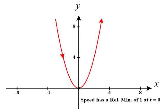
Example \(\PageIndex{4b}\)

Find any relative extrema in the speed function for the motion described by the parametric curve in Example \(\PageIndex{4a}\) above.

Solution

Since the speed function for this parameterized curve is

\(\text{Speed}(t) =\sqrt{1 + 4t^2},\)

the derivative of this function is

\(\text{Speed}'(t) =\dfrac{8t}{\sqrt{1 + 4t^2}}\).

Note that the denominator of this function is never \(0\) for this speed function, so there are no critical numbers where the function is defined but its derivative does not exist.  Checking for values of \(t\) where the derivative equals \(0\), we get the equation

\(\dfrac{8t}{\sqrt{1 + 4t^2}}=0\).

We see this only occurs when \(8t = 0\) or when \(t = 0\).  So \(t = 0\) is the only critical number of this speed function.

Using the first derivative test, we obtain the table below.

Intervals	Test Value, \(c\)	\(\text{Speed}'(c)\)	\(\text{Speed}(t)\) inc/dec	Interpretation
\((-\infty,0)\)	\(-1\)	\(\text{Speed}'(-1) =\dfrac{8(-1)}{\sqrt{1 + 4(-1)^2}}=\dfrac{-8}{\sqrt{5}}<0\)	\(\text{Speed}(t)\)  dec	\(\text{Speed}(t)\) has a relative min. at \(t = 0\).
\((0,\infty)\)	\(1\)	\(\text{Speed}'(1) =\dfrac{8(1)}{\sqrt{1 + 4(1)^2}}=\dfrac{8}{\sqrt{5}}>0\)	\(\text{Speed}(t)\)  inc

So we see that the speed of the motion along this parameterized curve will have a relative minimum at \(t=0\).  The value of this minimum speed will be

\(\text{Speed}(0) = \sqrt{1 + 4(0)^2} = \sqrt{1} = 1 \text{ unit per unit of time}\).

Note that based on the discussion above this example, we could have used the second derivative test on the radicand function to prove that the speed has a relative minimum at \(t=0\).

Example \(\PageIndex{5}\)

Find the speed of the motion along the following parameterized curve as a function of time \(t\) and determine any local extrema in this speed function.

\[x(t) = t^3-5t \quad y(t) = \frac{t^4}{2}\nonumber\]

Solution

First we find the derivatives of the component functions.

\[x'(t) = 3t^2-5 \quad y'(t) = 2t^3\nonumber\]

Then, using the formula for speed, we find

\[\begin{align*} \text{Speed}(t) &= \sqrt{(3t^2-5)^2 + (2t^3)^2} \\[4pt]
&=\sqrt{9t^4-30t^2+25 + 4t^6}\\[4pt]
&=\sqrt{4t^6+9t^4-30t^2+25}\end{align*}\]

Now

\(\text{Speed}'(t) =\dfrac{24t^5+36t^3-60t}{\sqrt{4t^6+9t^4-30t^2+25}}\).

As stated above, since a speed function is the square root of a sum of two squares, we can focus on finding critical numbers for the radicand (the function under the radical).  Let \(f(t) = 4t^6+9t^4-30t^2+25,\) the radicand from the original speed function. 

The derivative of the radicand is the numerator of the derivative shown above.

Setting this equal to zero we get

\(f'(t) = 24t^5+36t^3-60t = 0\)

We can factor the left side of this equation so we can use the zero-product property to solve it.

\(12t(2t^4+3t^2-5) = 0\)

\(12t(2t^2+5)(t^2-1) = 0\)

This equation has three real-valued solutions: \( t = 0, t = -1, t = 1\).  We don't need to find the two imaginary solutions for this situation, since they cannot be critical numbers.

Let's use the second derivative test to determine the nature of any relative extrema at these critical numbers.

\(f''(t) = 120t^4+108t^2-60\)

Then evaluating \(f''\) at each critical number we find

\[\begin{align*} f''(0) &= 120(0)^4+108(0)^2-60 = -60 < 0 && \text{So, }f\text{ is concave down, and so has a relative max at }t=0.\\[4pt]
f''(-1)&= 120(-1)^4+108(-1)^2-60 = 168 > 0 && \text{So, }f\text{ is concave up, and so has a relative min at }t=-1.\\[4pt]
f''(1)&= 120(1)^4+108(1)^2-60 = 168 > 0 && \text{So, }f\text{ is concave up, and so has a relative min at }t=1.  \end{align*}\]

Now to determine these relative extrema in the speed, we need to evaluate the speed function at each of these values of \(t\).

The motion determined by these parametric equations will have a relative maximum speed of

\[ \begin{align*} \text{Speed}(0) &= \sqrt{(3(0)^2-5)^2 + (2(0)^3)^2}\\[4pt]
&= \sqrt{25} = 5 \quad \text{ when } t = 0. \end{align*} \]

And the speed will have relative minima of

\[ \begin{align*} \text{Speed}(-1) &= \sqrt{(3(-1)^2-5)^2 + (2(-1)^3)^2}\\[4pt]
&= \sqrt{(-2)^2 + (-2)^2}\\[4pt]
&= \sqrt{8} = 2\sqrt{2} \quad \text{ when } t = -1. \end{align*} \]

and

\[ \begin{align*} \text{Speed}(1) &= \sqrt{(3(1)^2-5)^2 + (2(1)^3)^2}\\[4pt]
&= \sqrt{(-2)^2 + (2)^2}\\[4pt]
&= \sqrt{8} = 2\sqrt{2} \quad \text{ when } t = 1. \end{align*} \]

Figure \(\PageIndex{7}\): Graph of this parametric curve, showing the three points at which the speed is either a relative max or min.

Key Concepts

• The derivative of the parametrically defined curve \(x=x(t)\) and \(y=y(t)\) can be calculated using the formula \(\dfrac{dy}{dx}=\dfrac{y′(t)}{x′(t)}\). Using the derivative, we can find the equation of a tangent line to a parametric curve.

 

Key Equations

• Derivative of parametric equations

\[\dfrac{dy}{dx}=\dfrac{dy/dt}{dx/dt}=\dfrac{y′(t)}{x′(t)} \nonumber\]

• Second-order derivative of parametric equations

\[\dfrac{d^2y}{dx^2}=\dfrac{d}{dx}\left(\dfrac{dy}{dx}\right)=\dfrac{(d/dt)(dy/dx)}{dx/dt} \nonumber\]

• Speed of a Particle on a Parametric Curve \[ \text{Speed}(t) = \sqrt{\big(x'(t)\big)^2 + \big(y'(t)\big)^2}\nonumber\]

 

Contributors and Attributions

• Gilbert Strang (MIT) and Edwin “Jed” Herman (Harvey Mudd) with many contributing authors. This content by OpenStax is licensed with a CC-BY-SA-NC 4.0 license. Download for free at http://cnx.org.

• The subsection titled Speed along a Parametric Curve was written by Paul Seeburger (Monroe Community College).