
6.1: Areas between Curves
- Page ID
- 10830

- Determine the area of a region between two curves by integrating with respect to the independent variable.
- Find the area of a compound region.
- Determine the area of a region between two curves by integrating with respect to the dependent variable.
In Introduction to Integration, we developed the concept of the definite integral to calculate the area below a curve on a given interval. In this section, we expand that idea to calculate the area of more complex regions. We start by finding the area between two curves that are functions of \(\displaystyle x\), beginning with the simple case in which one function value is always greater than the other. We then look at cases when the graphs of the functions cross. Last, we consider how to calculate the area between two curves that are functions of \(\displaystyle y\).
Area of a Region between Two Curves
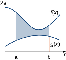
Let \(\displaystyle f(x)\) and \(\displaystyle g(x)\) be continuous functions over an interval \(\displaystyle [a,b]\) such that \(\displaystyle f(x)≥g(x)\) on \(\displaystyle [a,b]\). We want to find the area between the graphs of the functions, as shown in Figure \(\PageIndex{1}\).
As we did before, we are going to partition the interval on the x-axis and approximate the area between the graphs of the functions with rectangles. So, for \(\displaystyle i=0,1,2,…,n\), let \(\displaystyle P={x_i}\) be a regular partition of \(\displaystyle [a,b]\). Then, for \(\displaystyle i=1,2,…,n,\) choose a point \(\displaystyle x^∗_i∈[x_{i−1},x_i]\), and on each interval \(\displaystyle [x_{i−1},x_i]\) construct a rectangle that extends vertically from \(\displaystyle g(x^∗_i)\) to \(\displaystyle f(x^∗_i)\). Figure \(\PageIndex{2a}\) shows the rectangles when \(\displaystyle x^∗_i\) is selected to be the left endpoint of the interval and \(\displaystyle n=10\). Figure \(\PageIndex{2b}\) shows a representative rectangle in detail.
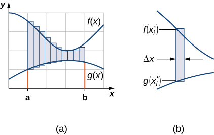
The height of each individual rectangle is \(\displaystyle f(x^∗_i)−g(x^∗_i)\) and the width of each rectangle is \(\displaystyle Δx\). Adding the areas of all the rectangles, we see that the area between the curves is approximated by
\[\displaystyle A≈\sum_{i=1}^n[f(x^∗_i)−g(x^∗_i)]Δx. \nonumber \]
This is a Riemann sum, so we take the limit as \(\displaystyle n→∞\) and we get
\[\displaystyle A=\lim_{n→∞}\sum_{i=1}^n[f(x^∗_i)−g(x^∗_i)]Δx=\int ^b_a[f(x)−g(x)]dx. \nonumber \]
These findings are summarized in the following theorem.
Let \(\displaystyle f(x)\) and \(\displaystyle g(x)\) be continuous functions such that \(\displaystyle f(x)≥g(x)\) over an interval [\(\displaystyle a,b]\). Let R denote the region bounded above by the graph of \(\displaystyle f(x)\), below by the graph of \(\displaystyle g(x)\), and on the left and right by the lines \(\displaystyle x=a\) and \(\displaystyle x=b\), respectively. Then, the area of \(\textbf{R}\) is given by
\[A=\int ^b_a[f(x)−g(x)]dx. \nonumber \]
We apply this theorem in the following example.
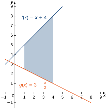
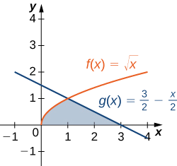
If \(\textbf{R}\) is the region bounded above by the graph of the function \(\displaystyle f(x)=x+4\) and below by the graph of the function \(\displaystyle g(x)=3−\dfrac{x}{2}\) over the interval \(\displaystyle [1,4]\), find the area of region \(\textbf{R}\).
Solution
The region is depicted in the following figure.
We have
\[ \begin{align*} A =\int ^b_a[f(x)−g(x)]\,dx \\[4pt] =\int ^4_1[(x+4)−(3−\dfrac{x}{2})]\,dx=\int ^4_1\left[\dfrac{3x}{2}+1\right]\,dx \\[4pt] =[\dfrac{3x^2}{4}+x]\bigg|^4_1=(16−\dfrac{7}{4})=\dfrac{57}{4}. \end{align*}\]
The area of the region is \(\displaystyle \dfrac{57}{4}units^2\).
If \(\textbf{R}\) is the region bounded by the graphs of the functions \(\displaystyle f(x)=\dfrac{x}{2}+5\) and \(\displaystyle g(x)=x+\dfrac{1}{2}\) over the interval \(\displaystyle [1,5]\), find the area of region \(\textbf{R}\).
- Hint
-
Graph the functions to determine which function’s graph forms the upper bound and which forms the lower bound, then follow the process used in Example.
- Answer
-
\(\displaystyle 12\) units2
In Example \(\PageIndex{1}\), we defined the interval of interest as part of the problem statement. Quite often, though, we want to define our interval of interest based on where the graphs of the two functions intersect. This is illustrated in the following example.
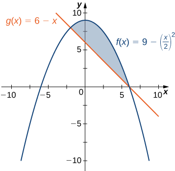
If \(\textbf{R}\) is the region bounded above by the graph of the function \(\displaystyle f(x)=9−(x/2)^2\) and below by the graph of the function \(\displaystyle g(x)=6−x\), find the area of region \(\textbf{R}\).
Solution
The region is depicted in the following figure.
We first need to compute where the graphs of the functions intersect. Setting \(\displaystyle f(x)=g(x),\) we get
\[ \begin{align*} \displaystyle f(x) =g(x) \\[4pt] 9−(\dfrac{x}{2})^2 =6−x\\[4pt] 9−\dfrac{x^2}{4} =6−x\\[4pt] 36−x^2 =24−4x\\[4pt] x^2−4x−12 =0\\[4pt] (x−6)(x+2) =0. \end{align*}\]
The graphs of the functions intersect when \(\displaystyle x=6\) or \(\displaystyle x=−2,\) so we want to integrate from \(\displaystyle −2\) to \(\displaystyle 6\). Since \(\displaystyle f(x)≥g(x)\) for \(\displaystyle −2≤x≤6,\) we obtain
\[\begin{align*} \displaystyle A =\int ^b_a[f(x)−g(x)]\,dx \\ =\int ^6_{−2} \left[9−(\dfrac{x}{2})^2−(6−x)\right]\,dx \\ =\int ^6_{−2}\left[3−\dfrac{x^2}{4}+x\right]\,dx \\ = \left. \left[3x−\dfrac{x^3}{12}+\dfrac{x^2}{2}\right] \right|^6_{−2}=\dfrac{64}{3}. \end{align*}\]
The area of the region is \(\displaystyle 64/3\) units2.
If \(\textbf{R}\) is the region bounded above by the graph of the function \(\displaystyle f(x)=x\) and below by the graph of the function \(\displaystyle g(x)=x^4\), find the area of region \(\textbf{R}\).
- Hint
-
Use the process from Example \(\PageIndex{2}\).
- Answer
-
\(\displaystyle \dfrac{3}{10}\) unit2
Areas of Compound Regions
So far, we have required \(\displaystyle f(x)≥g(x)\) over the entire interval of interest, but what if we want to look at regions bounded by the graphs of functions that cross one another? In that case, we modify the process we just developed by using the absolute value function.
Let \(\displaystyle f(x)\) and \(\displaystyle g(x)\) be continuous functions over an interval \(\displaystyle [a,b]\). Let \(\textbf{R}\) denote the region between the graphs of \(\displaystyle f(x)\) and \(\displaystyle g(x)\), and be bounded on the left and right by the lines \(\displaystyle x=a\) and \(\displaystyle x=b\), respectively. Then, the area of \(\textbf{R}\) is given by
\[A=\int ^b_a|f(x)−g(x)|dx. \nonumber \]
In practice, applying this theorem requires us to break up the interval \(\displaystyle [a,b]\) and evaluate several integrals, depending on which of the function values is greater over a given part of the interval. We study this process in the following example.
If \(\textbf{R}\) is the region between the graphs of the functions \(\displaystyle f(x)=\sin x \) and \(\displaystyle g(x)=\cos x\) over the interval \(\displaystyle [0,π]\), find the area of region \(\textbf{R}\).
Solution
The region is depicted in the following figure.
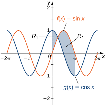
\(\displaystyle |f(x)−g(x)|=|\sin x −\cos x|=\cos x−\sin x .\)
On the other hand, for \(\displaystyle x∈[π/4,π], \sin x ≥\cos x,\) so
\(\displaystyle |f(x)−g(x)|=|\sin x −\cos x|=\sin x −\cos x.\)
Then
\[ \begin{align*} A =\int ^b_a|f(x)−g(x)|dx \\[4pt] =\int ^π_0|\sin x −\cos x|dx=\int ^{π/4}_0(\cos x−\sin x )dx+\int ^{π}_{π/4}(\sin x −\cos x)dx \\[4pt] =[\sin x +\cos x]|^{π/4}_0+[−\cos x−\sin x ]|^π_{π/4} \\[4pt] =(\sqrt{2}−1)+(1+\sqrt{2})=2\sqrt{2}. \end{align*}\]
The area of the region is \(\displaystyle 2\sqrt{2}\) units2.
If \(\textbf{R}\) is the region between the graphs of the functions \(\displaystyle f(x)=\sin x \) and \(\displaystyle g(x)=\cos x\) over the interval \(\displaystyle [π/2,2π]\), find the area of region \(\textbf{R}\).
- Hint
-
The two curves intersect at \(\displaystyle x=(5π)/4.\)
- Answer
-
\(\displaystyle 2+2\sqrt{2}\) units2
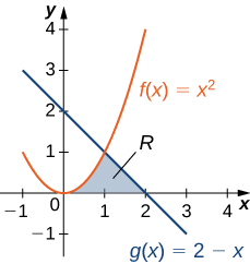
Consider the region depicted in Figure \(\PageIndex{6}\). Find the area of \(\textbf{R}\).

Solution
As with Example \(\PageIndex{3}\), we need to divide the interval into two pieces. The graphs of the functions intersect at \(\displaystyle x=1\) (set \(\displaystyle f(x)=g(x)\) and solve for x), so we evaluate two separate integrals: one over the interval \(\displaystyle [0,1]\) and one over the interval \(\displaystyle [1,2]\).
Over the interval \(\displaystyle [0,1]\), the region is bounded above by \(\displaystyle f(x)=x^2\) and below by the x-axis, so we have
\(\displaystyle A_1=\int ^1_0x^2dx=\dfrac{x^3}{3}∣^1_0=\dfrac{1}{3}.\)
Over the interval \(\displaystyle [1,2],\) the region is bounded above by \(\displaystyle g(x)=2−x\) and below by the x-axis, so we have
\(\displaystyle A_2=\int ^2_1(2−x)dx=[2x−\dfrac{x^2}{2}]∣^2_1=\dfrac{1}{2}.\)
Adding these areas together, we obtain
\(\displaystyle A=A_1+A_2=\dfrac{1}{3}+\dfrac{1}{2}=\dfrac{5}{6}.\)
The area of the region is \(\displaystyle 5/6\) units2.
Consider the region depicted in the following figure. Find the area of \(\textbf{R}\).
- Hint
-
The two curves intersect at x=1
- Answer
-
\(\displaystyle \dfrac{5}{3}\) units2
Regions Defined with Respect to y
In Example \(\PageIndex{4}\), we had to evaluate two separate integrals to calculate the area of the region. However, there is another approach that requires only one integral. What if we treat the curves as functions of \(\displaystyle y\), instead of as functions of \(\displaystyle x\)? Review Figure. Note that the left graph, shown in red, is represented by the function \(\displaystyle y=f(x)=x^2\). We could just as easily solve this for x and represent the curve by the function \(\displaystyle x=v(y)=\sqrt{y}\). (Note that \(\displaystyle x=−\sqrt{y}\) is also a valid representation of the function \(\displaystyle y=f(x)=x^2\) as a function of \(\displaystyle y\). However, based on the graph, it is clear we are interested in the positive square root.) Similarly, the right graph is represented by the function \(\displaystyle y=g(x)=2−x\), but could just as easily be represented by the function \(\displaystyle x=u(y)=2−y\). When the graphs are represented as functions of \(\displaystyle y\), we see the region is bounded on the left by the graph of one function and on the right by the graph of the other function. Therefore, if we integrate with respect to \(\displaystyle y\), we need to evaluate one integral only. Let’s develop a formula for this type of integration.
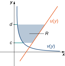
Let \(\displaystyle u(y)\) and \(\displaystyle v(y)\) be continuous functions over an interval \(\displaystyle [c,d]\) such that \(\displaystyle u(y)≥v(y)\) for all \(\displaystyle y∈[c,d]\). We want to find the area between the graphs of the functions, as shown in Figure \(\PageIndex{7}\).
This time, we are going to partition the interval on the y-axis and use horizontal rectangles to approximate the area between the functions. So, for \(\displaystyle i=0,1,2,…,n\), let \(\displaystyle Q={y_i}\) be a regular partition of \(\displaystyle [c,d]\). Then, for \(\displaystyle i=1,2,…,n\), choose a point \(\displaystyle y^∗_i∈[y_{i−1},y_i]\), then over each interval \(\displaystyle [y_{i−1},y_i]\) construct a rectangle that extends horizontally from \(\displaystyle v(y^0∗_i)\) to \(\displaystyle u(y^∗_i)\). Figure \(\PageIndex{8a}\)shows the rectangles when \(\displaystyle y^∗_i\) is selected to be the lower endpoint of the interval and \(\displaystyle n=10\). Figure \(\PageIndex{8b}\) shows a representative rectangle in detail.
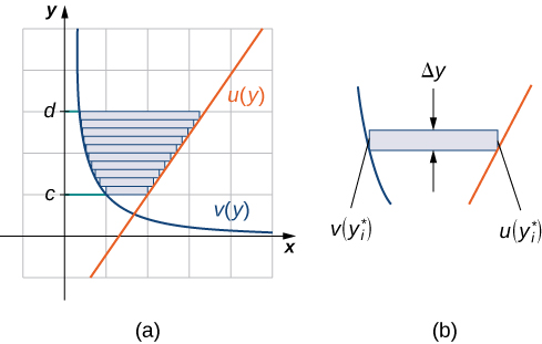
The height of each individual rectangle is \(\displaystyle Δy\) and the width of each rectangle is \(\displaystyle u(y^∗_i)−v(y^∗_i)\). Therefore, the area between the curves is approximately
\[ A≈\sum_{i=1}^n[u(y^∗_i)−v(y^∗_i)]Δy . \nonumber \]
This is a Riemann sum, so we take the limit as \(\displaystyle n→∞,\) obtaining
\[ \begin{align*} A =\lim_{n→∞}\sum_{i=1}^n[u(y^∗_i)−v(y^∗_i)]Δy \\[4pt] =\int ^d_c[u(y)−v(y)]dy. \end{align*}\]
These findings are summarized in the following theorem.
Let \(\displaystyle u(y)\) and \(\displaystyle v(y)\) be continuous functions such that \(\displaystyle u(y)≥v(y) \)for all \(\displaystyle y∈[c,d]\). Let \(\textbf{R}\) denote the region bounded on the right by the graph of \(\displaystyle u(y)\), on the left by the graph of \(\displaystyle v(y)\), and above and below by the lines \(\displaystyle y=d\) and \(\displaystyle y=c\), respectively. Then, the area of \(\textbf{R}\) is given by
\[A=\int ^d_c[u(y)−v(y)]dy. \nonumber \]
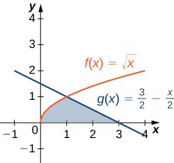
Let’s revisit Example \(\PageIndex{4}\), only this time let’s integrate with respect to \(\displaystyle y\). Let \(\textbf{R}\) be the region depicted in Figure \(\PageIndex{9}\). Find the area of \(\textbf{R}\) by integrating with respect to \(\displaystyle y\).
Solution
We must first express the graphs as functions of \(\displaystyle y\). As we saw at the beginning of this section, the curve on the left can be represented by the function \(\displaystyle x=v(y)=\sqrt{y}\), and the curve on the right can be represented by the function \(\displaystyle x=u(y)=2−y\).
Now we have to determine the limits of integration. The region is bounded below by the x-axis, so the lower limit of integration is \(\displaystyle y=0\). The upper limit of integration is determined by the point where the two graphs intersect, which is the point \(\displaystyle (1,1)\), so the upper limit of integration is \(\displaystyle y=1\). Thus, we have \(\displaystyle [c,d]=[0,1]\).
Calculating the area of the region, we get
\[ \begin{align*} A =\int ^d_c[u(y)−v(y)]dy \\[4pt] =\int ^1_0[(2−y)−\sqrt{y}]dy\\[4pt] =[2y−\dfrac{y^2}{2}−\dfrac{2}{3}y^{3/2}]∣^1_0\\[4pt] =\dfrac{5}{6}. \end{align*}\]
The area of the region is \(\displaystyle 5/6\) units2.
Let’s revisit the checkpoint associated with Example \(\PageIndex{4}\), only this time, let’s integrate with respect to \(\displaystyle y\). Let \(\textbf{R}\) be the region depicted in the following figure. Find the area of \(\textbf{R}\) by integrating with respect to \(\displaystyle y\).
- Hint
-
Follow the process from the previous example.
- Answer
-
\(\displaystyle \dfrac{5}{3}\) units2
Key Concepts
- Just as definite integrals can be used to find the area under a curve, they can also be used to find the area between two curves.
- To find the area between two curves defined by functions, integrate the difference of the functions.
- If the graphs of the functions cross, or if the region is complex, use the absolute value of the difference of the functions. In this case, it may be necessary to evaluate two or more integrals and add the results to find the area of the region.
- Sometimes it can be easier to integrate with respect to y to find the area. The principles are the same regardless of which variable is used as the variable of integration.
Key Equations
- Area between two curves, integrating on the x-axis
\(\displaystyle A=\int ^b_a[f(x)−g(x)]dx\)
- Area between two curves, integrating on the y-axis
\(\displaystyle A=\int ^d_c[u(y)−v(y)]dy\)