
6.3: Volumes of Revolution: The Shell Method
- Page ID
- 18172

\( \newcommand{\vecs}[1]{\overset { \scriptstyle \rightharpoonup} {\mathbf{#1}} } \)
\( \newcommand{\vecd}[1]{\overset{-\!-\!\rightharpoonup}{\vphantom{a}\smash {#1}}} \)
\( \newcommand{\dsum}{\displaystyle\sum\limits} \)
\( \newcommand{\dint}{\displaystyle\int\limits} \)
\( \newcommand{\dlim}{\displaystyle\lim\limits} \)
\( \newcommand{\id}{\mathrm{id}}\) \( \newcommand{\Span}{\mathrm{span}}\)
( \newcommand{\kernel}{\mathrm{null}\,}\) \( \newcommand{\range}{\mathrm{range}\,}\)
\( \newcommand{\RealPart}{\mathrm{Re}}\) \( \newcommand{\ImaginaryPart}{\mathrm{Im}}\)
\( \newcommand{\Argument}{\mathrm{Arg}}\) \( \newcommand{\norm}[1]{\| #1 \|}\)
\( \newcommand{\inner}[2]{\langle #1, #2 \rangle}\)
\( \newcommand{\Span}{\mathrm{span}}\)
\( \newcommand{\id}{\mathrm{id}}\)
\( \newcommand{\Span}{\mathrm{span}}\)
\( \newcommand{\kernel}{\mathrm{null}\,}\)
\( \newcommand{\range}{\mathrm{range}\,}\)
\( \newcommand{\RealPart}{\mathrm{Re}}\)
\( \newcommand{\ImaginaryPart}{\mathrm{Im}}\)
\( \newcommand{\Argument}{\mathrm{Arg}}\)
\( \newcommand{\norm}[1]{\| #1 \|}\)
\( \newcommand{\inner}[2]{\langle #1, #2 \rangle}\)
\( \newcommand{\Span}{\mathrm{span}}\) \( \newcommand{\AA}{\unicode[.8,0]{x212B}}\)
\( \newcommand{\vectorA}[1]{\vec{#1}} % arrow\)
\( \newcommand{\vectorAt}[1]{\vec{\text{#1}}} % arrow\)
\( \newcommand{\vectorB}[1]{\overset { \scriptstyle \rightharpoonup} {\mathbf{#1}} } \)
\( \newcommand{\vectorC}[1]{\textbf{#1}} \)
\( \newcommand{\vectorD}[1]{\overrightarrow{#1}} \)
\( \newcommand{\vectorDt}[1]{\overrightarrow{\text{#1}}} \)
\( \newcommand{\vectE}[1]{\overset{-\!-\!\rightharpoonup}{\vphantom{a}\smash{\mathbf {#1}}}} \)
\( \newcommand{\vecs}[1]{\overset { \scriptstyle \rightharpoonup} {\mathbf{#1}} } \)
\(\newcommand{\longvect}{\overrightarrow}\)
\( \newcommand{\vecd}[1]{\overset{-\!-\!\rightharpoonup}{\vphantom{a}\smash {#1}}} \)
\(\newcommand{\avec}{\mathbf a}\) \(\newcommand{\bvec}{\mathbf b}\) \(\newcommand{\cvec}{\mathbf c}\) \(\newcommand{\dvec}{\mathbf d}\) \(\newcommand{\dtil}{\widetilde{\mathbf d}}\) \(\newcommand{\evec}{\mathbf e}\) \(\newcommand{\fvec}{\mathbf f}\) \(\newcommand{\nvec}{\mathbf n}\) \(\newcommand{\pvec}{\mathbf p}\) \(\newcommand{\qvec}{\mathbf q}\) \(\newcommand{\svec}{\mathbf s}\) \(\newcommand{\tvec}{\mathbf t}\) \(\newcommand{\uvec}{\mathbf u}\) \(\newcommand{\vvec}{\mathbf v}\) \(\newcommand{\wvec}{\mathbf w}\) \(\newcommand{\xvec}{\mathbf x}\) \(\newcommand{\yvec}{\mathbf y}\) \(\newcommand{\zvec}{\mathbf z}\) \(\newcommand{\rvec}{\mathbf r}\) \(\newcommand{\mvec}{\mathbf m}\) \(\newcommand{\zerovec}{\mathbf 0}\) \(\newcommand{\onevec}{\mathbf 1}\) \(\newcommand{\real}{\mathbb R}\) \(\newcommand{\twovec}[2]{\left[\begin{array}{r}#1 \\ #2 \end{array}\right]}\) \(\newcommand{\ctwovec}[2]{\left[\begin{array}{c}#1 \\ #2 \end{array}\right]}\) \(\newcommand{\threevec}[3]{\left[\begin{array}{r}#1 \\ #2 \\ #3 \end{array}\right]}\) \(\newcommand{\cthreevec}[3]{\left[\begin{array}{c}#1 \\ #2 \\ #3 \end{array}\right]}\) \(\newcommand{\fourvec}[4]{\left[\begin{array}{r}#1 \\ #2 \\ #3 \\ #4 \end{array}\right]}\) \(\newcommand{\cfourvec}[4]{\left[\begin{array}{c}#1 \\ #2 \\ #3 \\ #4 \end{array}\right]}\) \(\newcommand{\fivevec}[5]{\left[\begin{array}{r}#1 \\ #2 \\ #3 \\ #4 \\ #5 \\ \end{array}\right]}\) \(\newcommand{\cfivevec}[5]{\left[\begin{array}{c}#1 \\ #2 \\ #3 \\ #4 \\ #5 \\ \end{array}\right]}\) \(\newcommand{\mattwo}[4]{\left[\begin{array}{rr}#1 \amp #2 \\ #3 \amp #4 \\ \end{array}\right]}\) \(\newcommand{\laspan}[1]{\text{Span}\{#1\}}\) \(\newcommand{\bcal}{\cal B}\) \(\newcommand{\ccal}{\cal C}\) \(\newcommand{\scal}{\cal S}\) \(\newcommand{\wcal}{\cal W}\) \(\newcommand{\ecal}{\cal E}\) \(\newcommand{\coords}[2]{\left\{#1\right\}_{#2}}\) \(\newcommand{\gray}[1]{\color{gray}{#1}}\) \(\newcommand{\lgray}[1]{\color{lightgray}{#1}}\) \(\newcommand{\rank}{\operatorname{rank}}\) \(\newcommand{\row}{\text{Row}}\) \(\newcommand{\col}{\text{Col}}\) \(\renewcommand{\row}{\text{Row}}\) \(\newcommand{\nul}{\text{Nul}}\) \(\newcommand{\var}{\text{Var}}\) \(\newcommand{\corr}{\text{corr}}\) \(\newcommand{\len}[1]{\left|#1\right|}\) \(\newcommand{\bbar}{\overline{\bvec}}\) \(\newcommand{\bhat}{\widehat{\bvec}}\) \(\newcommand{\bperp}{\bvec^\perp}\) \(\newcommand{\xhat}{\widehat{\xvec}}\) \(\newcommand{\vhat}{\widehat{\vvec}}\) \(\newcommand{\uhat}{\widehat{\uvec}}\) \(\newcommand{\what}{\widehat{\wvec}}\) \(\newcommand{\Sighat}{\widehat{\Sigma}}\) \(\newcommand{\lt}{<}\) \(\newcommand{\gt}{>}\) \(\newcommand{\amp}{&}\) \(\definecolor{fillinmathshade}{gray}{0.9}\)Often a given problem can be solved in more than one way. A particular method may be chosen out of convenience, personal preference, or perhaps necessity. Ultimately, it is good to have options.
The previous section introduced the Disk and Washer Methods, which computed the volume of solids of revolution by integrating the cross--sectional area of the solid. This section develops another method of computing volume, the Shell Method. Instead of slicing the solid perpendicular to the axis of rotation creating cross-sections, we now slice it parallel to the axis of rotation, creating "shells."
Consider Figure \(\PageIndex{1}\), where the region shown in (a) is rotated around the \(y\)-axis forming the solid shown in (b). A small slice of the region is drawn in (a), parallel to the axis of rotation. When the region is rotated, this thin slice forms a cylindrical shell, as pictured in part (c) of the figure. The previous section approximated a solid with lots of thin disks (or washers); we now approximate a solid with many thin cylindrical shells.
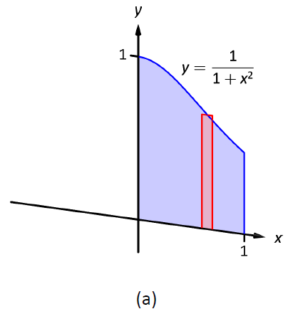
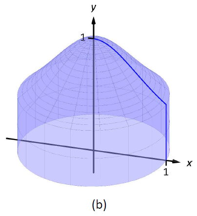
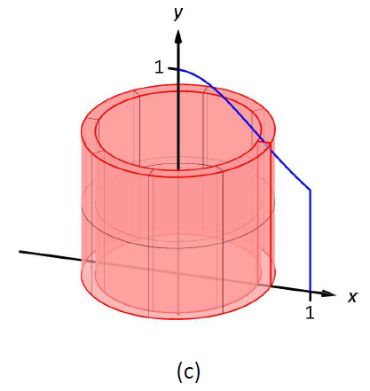
Figure \(\PageIndex{1}\): Introducing the Shell Method.
Figure \(\PageIndex{1}\)(d): A dynamic version of this figure created using CalcPlot3D.
To compute the volume of one shell, first consider the paper label on a soup can with radius \(r\) and height \(h\). What is the area of this label? A simple way of determining this is to cut the label and lay it out flat, forming a rectangle with height \(h\) and length \(2\pi r\). Thus the area is \(A = 2\pi rh\); see Figure \(\PageIndex{2a}\).
Do a similar process with a cylindrical shell, with height \(h\), thickness \(\Delta x\), and approximate radius \(r\). Cutting the shell and laying it flat forms a rectangular solid with length \(2\pi r\), height \(h\) and depth \(dx\). Thus the volume is \(V \approx 2\pi rh\ dx\); see Figure \(\PageIndex{2c}\). (We say "approximately" since our radius was an approximation.)
By breaking the solid into \(n\) cylindrical shells, we can approximate the volume of the solid as
$$V = \sum_{i=1}^n 2\pi r_ih_i\ dx_i,$$
where \(r_i\), \(h_i\) and \(dx_i\) are the radius, height and thickness of the \(i\,^\text{th}\) shell, respectively.
This is a Riemann Sum. Taking a limit as the thickness of the shells approaches 0 leads to a definite integral.
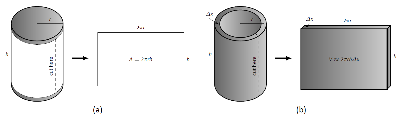
Figure \(\PageIndex{2}\): Determining the volume of a thin cylindrical shell.}\label{fig:soupcan}
Key Idea 25: Shell Method
Let a solid be formed by revolving a region \(R\), bounded by \(x=a\) and \(x=b\), around a vertical axis. Let \(r(x)\) represent the distance from the axis of rotation to \(x\) (i.e., the radius of a sample shell) and let \(h(x)\) represent the height of the solid at \(x\) (i.e., the height of the shell). The volume of the solid is
$$V = 2\pi\int_a^b r(x)h(x)\ dx.$$
Special Cases:
- When the region \(R\) is bounded above by \(y=f(x)\) and below by \(y=g(x)\), then \(h(x) = f(x)-g(x)\).
- When the axis of rotation is the \(y\)-axis (i.e., \(x=0\)) then \(r(x) = x\).
Let's practice using the Shell Method.
Example \(\PageIndex{1}\): Finding volume using the Shell Method
Find the volume of the solid formed by rotating the region bounded by \(y=0\), \(y=1/(1+x^2)\), \(x=0\) and \(x=1\) about the \(y\)-axis.
Solution
This is the region used to introduce the Shell Method in Figure \(\PageIndex{1}\), but is sketched again in Figure \(\PageIndex{3}\) for closer reference. A line is drawn in the region parallel to the axis of rotation representing a shell that will be carved out as the region is rotated about the \(y\)-axis. (This is the differential element.)
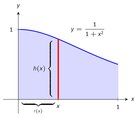
Figure \(\PageIndex{3}\): Graphing a region in Example \(\PageIndex{1}\).
The distance this line is from the axis of rotation determines \(r(x)\); as the distance from \(x\) to the \(y\)-axis is \(x\), we have \(r(x)=x\). The height of this line determines \(h(x)\); the top of the line is at \(y=1/(1+x^2)\), whereas the bottom of the line is at \(y=0\). Thus \(h(x) = 1/(1+x^2)-0 = 1/(1+x^2)\). The region is bounded from \(x=0\) to \(x=1\), so the volume is
\[V = 2\pi\int_0^1 \dfrac{x}{1+x^2}\ dx.\]
This requires substitution. Let \(u=1+x^2\), so \(du = 2x\ dx\). We also change the bounds: \(u(0) = 1\) and \(u(1) = 2\). Thus we have:
\[\begin{align*} &= \pi\int_1^2 \dfrac{1}{u}\ du \\[5pt] &= \pi\ln u\Big|_1^2\\[5pt] &= \pi\ln 2 - \pi\ln 1\\[5pt] &= \pi\ln 2 \approx 2.178 \ \text{units}^3.\end{align*}\]
Note: in order to find this volume using the Disk Method, two integrals would be needed to account for the regions above and below \(y=1/2\).
With the Shell Method, nothing special needs to be accounted for to compute the volume of a solid that has a hole in the middle, as demonstrated next.
Example \(\PageIndex{2}\): Finding volume using the Shell Method
Find the volume of the solid formed by rotating the triangular region determined by the points \((0,1)\), \((1,1)\) and \((1,3)\) about the line \(x=3\).
Solution
The region is sketched in Figure \(\PageIndex{4a}\) along with the differential element, a line within the region parallel to the axis of rotation. In part (b) of the figure, we see the shell traced out by the differential element, and in part (c) the whole solid is shown.
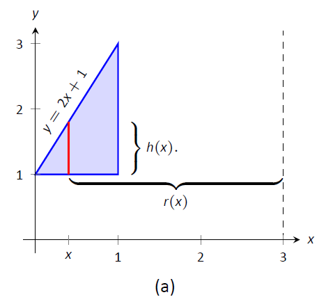
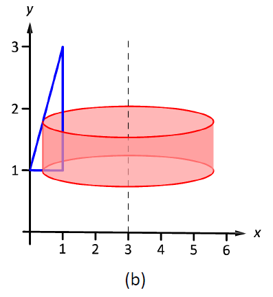
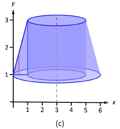
Figure \(\PageIndex{4}\): Graphing a region in Example \(\PageIndex{2}\)
The height of the differential element is the distance from \(y=1\) to \(y=2x+1\), the line that connects the points \((0,1)\) and \((1,3)\). Thus \(h(x) = 2x+1-1 = 2x\). The radius of the shell formed by the differential element is the distance from \(x\) to \(x=3\); that is, it is \(r(x)=3-x\). The \(x\)-bounds of the region are \(x=0\) to \(x=1\), giving
\[\begin{align*} V &= 2\pi\int_0^1 (3-x)(2x)\ dx \\[5pt] &= 2\pi\int_0^1 \big(6x-2x^2)\ dx \\[5pt] &= 2\pi\left(3x^2-\dfrac23x^3\right)\Big|_0^1\\[5pt] &= \dfrac{14}{3}\pi\approx 14.66 \ \text{units}^3.\end{align*}\]
When revolving a region around a horizontal axis, we must consider the radius and height functions in terms of \(y\), not \(x\).
Example \(\PageIndex{3}\): Finding volume using the Shell Method
Find the volume of the solid formed by rotating the region given in Example \(\PageIndex{2}\) about the \(x\)-axis.
Solution
The region is sketched in Figure \(\PageIndex{5a}\) with a sample differential element. In part (b) of the figure the shell formed by the differential element is drawn, and the solid is sketched in (c). (Note that the triangular region looks "short and wide" here, whereas in the previous example the same region looked "tall and narrow." This is because the bounds on the graphs are different.)
The height of the differential element is an \(x\)-distance, between \(x=\dfrac12y-\dfrac12\) and \(x=1\). Thus \(h(y) = 1-(\dfrac12y-\dfrac12) = -\dfrac12y+\dfrac32.\) The radius is the distance from \(y\) to the \(x\)-axis, so \(r(y) =y\). The \(y\) bounds of the region are \(y=1\) and \(y=3\), leading to the integral
\[\begin{align*}V &= 2\pi\int_1^3\left[y\left(-\dfrac12y+\dfrac32\right)\right]\ dy \\[5pt]&= 2\pi\int_1^3\left[-\dfrac12y^2+\dfrac32y\right]\ dy \\[5pt] &= 2\pi\left[-\dfrac16y^3+\dfrac34y^2\right]\Big|_1^3 \\[5pt] &= 2\pi\left[\dfrac94-\dfrac7{12}\right]\\[5pt] &= \dfrac{10}{3}\pi \approx 10.472\ \text{units}^3.\end{align*}\]
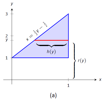
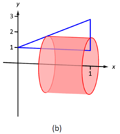
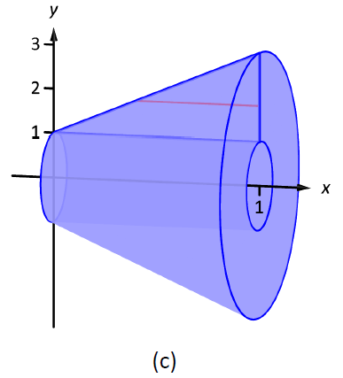
Figure \(\PageIndex{5}\): Graphing a region in Example \(\PageIndex{3}\)
At the beginning of this section it was stated that "it is good to have options." The next example finds the volume of a solid rather easily with the Shell Method, but using the Washer Method would be quite a chore.
Example \(\PageIndex{4}\): Finding volume using the Shell Method
Find the volume of the solid formed by revolving the region bounded by \(y= \sin x\) and the \(x\)-axis from \(x=0\) to \(x=\pi\) about the \(y\)-axis.
Solution
The region and a differential element, the shell formed by this differential element, and the resulting solid are given in Figure \(\PageIndex{6}\).
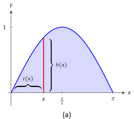
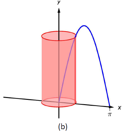
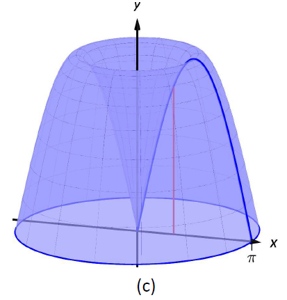
Figure \(\PageIndex{6}a\): Graphing a region in Example \(\PageIndex{4}\)
Figure \(\PageIndex{6}b\): Visualizing this figure using CalcPlot3D
The radius of a sample shell is \(r(x) = x\); the height of a sample shell is \(h(x) = \sin x\), each from \(x=0\) to \(x=\pi\). Thus the volume of the solid is
\[V = 2\pi\int_0^{\pi} x\sin x\ dx.\]
This requires Integration By Parts. Set \(u=x\) and \(dv=\sin x\ dx\); we leave it to the reader to fill in the rest. We have:
\[\begin{align*} &= 2\pi\Big[-x\cos x\Big|_0^{\pi} +\int_0^{\pi}\cos x\ dx \Big] \\[5pt]
&= 2\pi\Big[\pi + \sin x \Big|_0^{\pi}\ \Big] \\[5pt]
&= 2\pi\Big[\pi + 0 \Big] \\[5pt]
&= 2\pi^2 \approx 19.74 \ \text{units}^3. \end{align*}\]
Note that in order to use the Washer Method, we would need to solve \(y=\sin x\) for \(x\), requiring the use of the arcsine function. We leave it to the reader to verify that the outside radius function is \(R(y) = \pi-\arcsin y\) and the inside radius function is \(r(y)=\arcsin y\). Thus the volume can be computed as
$$\pi\int_0^1 \Big[ (\pi-\arcsin y)^2-(\arcsin y)^2\Big]\ dy.$$
This integral isn't terrible given that the \(\arcsin^2 y\) terms cancel, but it is more onerous than the integral created by the Shell Method.
We end this section with a table summarizing the usage of the Washer and Shell Methods.
Key Idea 26: Summary of the Washer and Shell Methods
Let a region \(R\) be given with \(x\)-bounds \(x=a\) and \(x=b\) and \(y\)-bounds \(y=c\) and \(y=d\).
\[\begin{align*} & \text{Washer Method} & & \text{Shell Method} \\[5pt] \text{Horizontal Axis} \quad & \pi\int_a^b \big(R(x)^2-r(x)^2\big)\ dx & & 2\pi\int_c^d r(y)h(y)\ dy \\[5pt] \\[5pt] \text{Vertical Axis} \quad & \pi \int_c^d\big(R(y)^2-r(y)^2\big)\ dy & & 2\pi\int_a^b r(x)h(x)\ dx \end{align*}\]
As in the previous section, the real goal of this section is not to be able to compute volumes of certain solids. Rather, it is to be able to solve a problem by first approximating, then using limits to refine the approximation to give the exact value. In this section, we approximate the volume of a solid by cutting it into thin cylindrical shells. By summing up the volumes of each shell, we get an approximation of the volume. By taking a limit as the number of equally spaced shells goes to infinity, our summation can be evaluated as a definite integral, giving the exact value.
We use this same principle again in the next section, where we find the length of curves in the plane.
Contributors
Gregory Hartman (Virginia Military Institute). Contributions were made by Troy Siemers and Dimplekumar Chalishajar of VMI and Brian Heinold of Mount Saint Mary's University. This content is copyrighted by a Creative Commons Attribution - Noncommercial (BY-NC) License. http://www.apexcalculus.com/
Integrated by Justin Marshall.