10.4: Working with Taylor Series

Learning Objectives

• Write the terms of the binomial series.
• Recognize the Taylor series expansions of common functions.
• Recognize and apply techniques to find the Taylor series for a function.
• Use Taylor series to solve differential equations.
• Use Taylor series to evaluate non-elementary integrals.

In the preceding section, we defined Taylor series and showed how to find the Taylor series for several common functions by explicitly calculating the coefficients of the Taylor polynomials. In this section we show how to use those Taylor series to derive Taylor series for other functions. We then present two common applications of power series. First, we show how power series can be used to solve differential equations. Second, we show how power series can be used to evaluate integrals when the antiderivative of the integrand cannot be expressed in terms of elementary functions. In one example, we consider an integral that arises frequently in probability theory.

The Binomial Series

Our first goal in this section is to determine the Maclaurin series for the function for all real numbers . The Maclaurin series for this function is known as the binomial series. We begin by considering the simplest case: is a nonnegative integer. We recall that, for can be written as

The expressions on the right-hand side are known as binomial expansions and the coefficients are known as binomial coefficients. More generally, for any nonnegative integer , the binomial coefficient of in the binomial expansion of is given by

and

For example, using this formula for , we see that

We now consider the case when the exponent is any real number, not necessarily a nonnegative integer. If is not a nonnegative integer, then cannot be written as a finite polynomial. However, we can find a power series for . Specifically, we look for the Maclaurin series for . To do this, we find the derivatives of and evaluate them at .

We conclude that the coefficients in the binomial series are given by

We note that if is a nonnegative integer, then the derivative is the zero function, and the series terminates. In addition, if is a nonnegative integer, then Equation   for the coefficients agrees with Equation   for the coefficients, and the formula for the binomial series agrees with Equation   for the finite binomial expansion. More generally, to denote the binomial coefficients for any real number , we define

With this notation, we can write the binomial series for as

We now need to determine the interval of convergence for the binomial series Equation . We apply the ratio test. Consequently, we consider

.

Since

if and only if , we conclude that the interval of convergence for the binomial series is . The behavior at the endpoints depends on . It can be shown that for the series converges at both endpoints; for , the series converges at and diverges at ; and for , the series diverges at both endpoints. The binomial series does converge to in for all real numbers , but proving this fact by showing that the remainder is difficult.

Definition: Binomial Series

For any real number , the Maclaurin series for is the binomial series. It converges to for , and we write

for .

We can use this definition to find the binomial series for and use the series to approximate .

Example : Finding Binomial Series

1. Find the binomial series for .
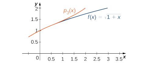
2. Use the third-order Maclaurin polynomial to estimate . Use Taylor’s theorem to bound the error. Use a graphing utility to compare the graphs of and .

Solution

a. Here . Using the definition for the binomial series, we obtain

b. From the result in part a. the third-order Maclaurin polynomial is

.

Therefore,

From Taylor’s theorem, the error satisfies

for some between and . Since , and the maximum value of on the interval occurs at , we have

The function and the Maclaurin polynomial are graphed in Figure .

Figure : The third-order Maclaurin polynomial provides a good approximation for for near zero.

Exercise

Find the binomial series for .

Hint

Use the definition of binomial series for .

Answer

Common Functions Expressed as Taylor Series

At this point, we have derived Maclaurin series for exponential, trigonometric, and logarithmic functions, as well as functions of the form . In Table , we summarize the results of these series. We remark that the convergence of the Maclaurin series for at the endpoint and the Maclaurin series for at the endpoints and relies on a more advanced theorem than we present here. (Refer to Abel’s theorem for a discussion of this more technical point.)

Table : Maclaurin Series for Common Functions

Function	Maclaurin Series	Interval of Convergence
		Convergence at the endpoints depends on the value of

Earlier in the chapter, we showed how you could combine power series to create new power series. Here we use these properties, combined with the Maclaurin series in Table , to create Maclaurin series for other functions.

Example : Deriving Maclaurin Series from Known Series

Find the Maclaurin series of each of the following functions by using one of the series listed in Table .

Solution

a. Using the Maclaurin series for we find that the Maclaurin series for is given by

This series converges to for all in the domain of ; that is, for all .

b. To find the Maclaurin series for we use the fact that

Using the Maclaurin series for , we see that the term in the Maclaurin series for is given by

For even, this term is zero. For odd, this term is . Therefore, the Maclaurin series for has only odd-order terms and is given by

Exercise

Find the Maclaurin series for

Hint

Use the Maclaurin series for

Answer

We also showed previously in this chapter how power series can be differentiated term by term to create a new power series. In Example , we differentiate the binomial series for term by term to find the binomial series for . Note that we could construct the binomial series for directly from the definition, but differentiating the binomial series for is an easier calculation.

Example : Differentiating a Series to Find a New Series

Use the binomial series for to find the binomial series for .

Solution

The two functions are related by

,

so the binomial series for is given by

Exercise

Find the binomial series for

Hint

Differentiate the series for

Answer

In this example, we differentiated a known Taylor series to construct a Taylor series for another function. The ability to differentiate power series term by term makes them a powerful tool for solving differential equations. We now show how this is accomplished.

Solving Differential Equations with Power Series

Consider the differential equation

Recall that this is a first-order separable equation and its solution is . This equation is easily solved using techniques discussed earlier in the text. For most differential equations, however, we do not yet have analytical tools to solve them. Power series are an extremely useful tool for solving many types of differential equations. In this technique, we look for a solution of the form and determine what the coefficients would need to be. In the next example, we consider an initial-value problem involving to illustrate the technique.

Example : Power Series Solution of a Differential Equation

Use power series to solve the initial-value problem

Solution

Suppose that there exists a power series solution

Differentiating this series term by term, we obtain

If satisfies the differential equation, then

Using the uniqueness of power series representations, we know that these series can only be equal if their coefficients are equal. Therefore,

⋮

Using the initial condition combined with the power series representation

,

we find that . We are now ready to solve for the rest of the coefficients. Using the fact that , we have

Therefore,

You might recognize

as the Taylor series for . Therefore, the solution is .

Exercise

Use power series to solve

Hint

The equations for the first several coefficients will satisfy In general, for all .

Answer

We now consider an example involving a differential equation that we cannot solve using previously discussed methods. This differential equation

is known as Airy’s equation. It has many applications in mathematical physics, such as modeling the diffraction of light. Here we show how to solve it using power series.

Example : Power Series Solution of Airy’s Equation

Use power series to solve with the initial conditions and

Solution

We look for a solution of the form

Differentiating this function term by term, we obtain

If satisfies the equation , then

Using the Uniqueness of Power Series Theorem (from an earlier Section) on the uniqueness of power series representations, we know that coefficients of the same degree must be equal. Therefore,

⋮

More generally, for , we have . In fact, all coefficients can be written in terms of and . To see this, first note that . Then

,

.

For , we see that

Therefore, the series solution of the differential equation is given by

The initial condition implies . Differentiating this series term by term and using the fact that , we conclude that .

Therefore, the solution of this initial-value problem is

Exercise

Use power series to solve with the initial condition and .

Hint

The coefficients satisfy and for .

Answer

Evaluating Non-elementary Integrals

Solving differential equations is one common application of power series. We now turn to a second application. We show how power series can be used to evaluate integrals involving functions whose antiderivatives cannot be expressed using elementary functions.

One integral that arises often in applications in probability theory is Unfortunately, the antiderivative of the integrand is not an elementary function. By elementary function, we mean a function that can be written using a finite number of algebraic combinations or compositions of exponential, logarithmic, trigonometric, or power functions. We remark that the term “elementary function” is not synonymous with noncomplicated function. For example, the function is an elementary function, although not a particularly simple-looking function. Any integral of the form where the antiderivative of cannot be written as an elementary function is considered a non-elementary integral.

Non-elementary integrals cannot be evaluated using the basic integration techniques discussed earlier. One way to evaluate such integrals is by expressing the integrand as a power series and integrating term by term. We demonstrate this technique by considering

Example : Using Taylor Series to Evaluate a Definite Integral

1. Express as an infinite series.
2. Evaluate to within an error of .

Solution

a. The Maclaurin series for is given by

Therefore,

b. Using the result from part a. we have

The sum of the first four terms is approximately . By the alternating series test, this estimate is accurate to within an error of less than

Exercise

Express as an infinite series. Evaluate to within an error of .

Hint

Use the series found in Example .

Answer

The definite integral is approximately to within an error of .

As mentioned above, the integral arises often in probability theory. Specifically, it is used when studying data sets that are normally distributed, meaning the data values lie under a bell-shaped curve. For example, if a set of data values is normally distributed with mean and standard deviation , then the probability that a randomly chosen value lies between and is given by

(See Figure .)

Figure : If data values are normally distributed with mean and standard deviation , the probability that a randomly selected data value is between and is the area under the curve between and .

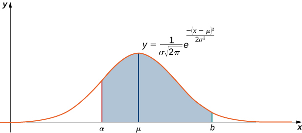
To simplify this integral, we typically let . This quantity is known as the score of a data value. With this simplification, integral Equation becomes

In Example , we show how we can use this integral in calculating probabilities.

Example : Using Maclaurin Series to Approximate a Probability

Suppose a set of standardized test scores are normally distributed with mean and standard deviation . Use Equation and the first six terms in the Maclaurin series for to approximate the probability that a randomly selected test score is between and . Use the alternating series test to determine how accurate your approximation is.

Solution

Since and we are trying to determine the area under the curve from to , integral Equation becomes

The Maclaurin series for is given by

Therefore,

We now use this result to evaluate the definite integral from Equation :

Using the first five terms, we estimate that the probability is approximately 0.4729. By the alternating series test, we see that this estimate is accurate to within

Analysis

If you are familiar with probability theory, you may know that the probability that a data value is within two standard deviations of the mean is approximately Here we calculated the probability that a data value is between the mean and two standard deviations above the mean, so the estimate should be around . The estimate, combined with the bound on the accuracy, falls within this range.

Alternative method. If term-by-term integration is done instead, the result of evaluating the definite integral is

Exercise

Given a set of normally distributed standardized test scores with mean and standard deviation , use the first five terms of the Maclaurin series for to estimate the probability that a randomly selected test score is between and . Use the alternating series test to determine the accuracy of this estimate.

Hint

Evaluate using the first five terms of the Maclaurin series for .

Answer

The estimate is approximately This estimate is accurate to within

Another application in which a non-elementary integral arises involves the period of a pendulum. The integral is

.

An integral of this form is known as an elliptic integral of the first kind. Elliptic integrals originally arose when trying to calculate the arc length of an ellipse. We now show how to use power series to approximate this integral.

Example : Period of a Pendulum

The period of a pendulum is the time it takes for a pendulum to make one complete back-and-forth swing. For a pendulum with length that makes a maximum angle with the vertical, its period is given by

where is the acceleration due to gravity and (see Figure ). (We note that this formula for the period arises from a non-linearized model of a pendulum. In some cases, for simplification, a linearized model is used and is approximated by .)

Figure : This pendulum has length and makes a maximum angle with the vertical.

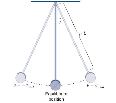
Use the binomial series

to estimate the period of this pendulum. Specifically, approximate the period of the pendulum if

1. you use only the first term in the binomial series, and
2. you use the first two terms in the binomial series.

Solution

We use the binomial series, replacing x with Then we can write the period as

a. Using just the first term in the integrand, the first-order estimate is

If is small, then is small. We claim that when is small, this is a good estimate. To justify this claim, consider

Since , this integral is bounded by

Furthermore, it can be shown that each coefficient on the right-hand side is less than and, therefore, that this expression is bounded by

,

which is small for small.

b. For larger values of , we can approximate by using more terms in the integrand. By using the first two terms in the integral, we arrive at the estimate

The applications of Taylor series in this section are intended to highlight their importance. In general, Taylor series are useful because they allow us to represent known functions using polynomials, thus providing us a tool for approximating function values and estimating complicated integrals. In addition, they allow us to define new functions as power series, thus providing us with a powerful tool for solving differential equations.

Key Concepts

• The binomial series is the Maclaurin series for . It converges for .
• Taylor series for functions can often be derived by algebraic operations with a known Taylor series or by differentiating or integrating a known Taylor series.
• Power series can be used to solve differential equations.
• Taylor series can be used to help approximate integrals that cannot be evaluated by other means.

Glossary

binomial series

the Maclaurin series for ; it is given by for

non-elementary integral

an integral for which the antiderivative of the integrand cannot be expressed as an elementary function