
13.2: Limits and Continuity
- Page ID
- 9041
\( \newcommand{\vecs}[1]{\overset { \scriptstyle \rightharpoonup} {\mathbf{#1}} } \)
\( \newcommand{\vecd}[1]{\overset{-\!-\!\rightharpoonup}{\vphantom{a}\smash {#1}}} \)
\( \newcommand{\id}{\mathrm{id}}\) \( \newcommand{\Span}{\mathrm{span}}\)
( \newcommand{\kernel}{\mathrm{null}\,}\) \( \newcommand{\range}{\mathrm{range}\,}\)
\( \newcommand{\RealPart}{\mathrm{Re}}\) \( \newcommand{\ImaginaryPart}{\mathrm{Im}}\)
\( \newcommand{\Argument}{\mathrm{Arg}}\) \( \newcommand{\norm}[1]{\| #1 \|}\)
\( \newcommand{\inner}[2]{\langle #1, #2 \rangle}\)
\( \newcommand{\Span}{\mathrm{span}}\)
\( \newcommand{\id}{\mathrm{id}}\)
\( \newcommand{\Span}{\mathrm{span}}\)
\( \newcommand{\kernel}{\mathrm{null}\,}\)
\( \newcommand{\range}{\mathrm{range}\,}\)
\( \newcommand{\RealPart}{\mathrm{Re}}\)
\( \newcommand{\ImaginaryPart}{\mathrm{Im}}\)
\( \newcommand{\Argument}{\mathrm{Arg}}\)
\( \newcommand{\norm}[1]{\| #1 \|}\)
\( \newcommand{\inner}[2]{\langle #1, #2 \rangle}\)
\( \newcommand{\Span}{\mathrm{span}}\) \( \newcommand{\AA}{\unicode[.8,0]{x212B}}\)
\( \newcommand{\vectorA}[1]{\vec{#1}} % arrow\)
\( \newcommand{\vectorAt}[1]{\vec{\text{#1}}} % arrow\)
\( \newcommand{\vectorB}[1]{\overset { \scriptstyle \rightharpoonup} {\mathbf{#1}} } \)
\( \newcommand{\vectorC}[1]{\textbf{#1}} \)
\( \newcommand{\vectorD}[1]{\overrightarrow{#1}} \)
\( \newcommand{\vectorDt}[1]{\overrightarrow{\text{#1}}} \)
\( \newcommand{\vectE}[1]{\overset{-\!-\!\rightharpoonup}{\vphantom{a}\smash{\mathbf {#1}}}} \)
\( \newcommand{\vecs}[1]{\overset { \scriptstyle \rightharpoonup} {\mathbf{#1}} } \)
\( \newcommand{\vecd}[1]{\overset{-\!-\!\rightharpoonup}{\vphantom{a}\smash {#1}}} \)
\(\newcommand{\avec}{\mathbf a}\) \(\newcommand{\bvec}{\mathbf b}\) \(\newcommand{\cvec}{\mathbf c}\) \(\newcommand{\dvec}{\mathbf d}\) \(\newcommand{\dtil}{\widetilde{\mathbf d}}\) \(\newcommand{\evec}{\mathbf e}\) \(\newcommand{\fvec}{\mathbf f}\) \(\newcommand{\nvec}{\mathbf n}\) \(\newcommand{\pvec}{\mathbf p}\) \(\newcommand{\qvec}{\mathbf q}\) \(\newcommand{\svec}{\mathbf s}\) \(\newcommand{\tvec}{\mathbf t}\) \(\newcommand{\uvec}{\mathbf u}\) \(\newcommand{\vvec}{\mathbf v}\) \(\newcommand{\wvec}{\mathbf w}\) \(\newcommand{\xvec}{\mathbf x}\) \(\newcommand{\yvec}{\mathbf y}\) \(\newcommand{\zvec}{\mathbf z}\) \(\newcommand{\rvec}{\mathbf r}\) \(\newcommand{\mvec}{\mathbf m}\) \(\newcommand{\zerovec}{\mathbf 0}\) \(\newcommand{\onevec}{\mathbf 1}\) \(\newcommand{\real}{\mathbb R}\) \(\newcommand{\twovec}[2]{\left[\begin{array}{r}#1 \\ #2 \end{array}\right]}\) \(\newcommand{\ctwovec}[2]{\left[\begin{array}{c}#1 \\ #2 \end{array}\right]}\) \(\newcommand{\threevec}[3]{\left[\begin{array}{r}#1 \\ #2 \\ #3 \end{array}\right]}\) \(\newcommand{\cthreevec}[3]{\left[\begin{array}{c}#1 \\ #2 \\ #3 \end{array}\right]}\) \(\newcommand{\fourvec}[4]{\left[\begin{array}{r}#1 \\ #2 \\ #3 \\ #4 \end{array}\right]}\) \(\newcommand{\cfourvec}[4]{\left[\begin{array}{c}#1 \\ #2 \\ #3 \\ #4 \end{array}\right]}\) \(\newcommand{\fivevec}[5]{\left[\begin{array}{r}#1 \\ #2 \\ #3 \\ #4 \\ #5 \\ \end{array}\right]}\) \(\newcommand{\cfivevec}[5]{\left[\begin{array}{c}#1 \\ #2 \\ #3 \\ #4 \\ #5 \\ \end{array}\right]}\) \(\newcommand{\mattwo}[4]{\left[\begin{array}{rr}#1 \amp #2 \\ #3 \amp #4 \\ \end{array}\right]}\) \(\newcommand{\laspan}[1]{\text{Span}\{#1\}}\) \(\newcommand{\bcal}{\cal B}\) \(\newcommand{\ccal}{\cal C}\) \(\newcommand{\scal}{\cal S}\) \(\newcommand{\wcal}{\cal W}\) \(\newcommand{\ecal}{\cal E}\) \(\newcommand{\coords}[2]{\left\{#1\right\}_{#2}}\) \(\newcommand{\gray}[1]{\color{gray}{#1}}\) \(\newcommand{\lgray}[1]{\color{lightgray}{#1}}\) \(\newcommand{\rank}{\operatorname{rank}}\) \(\newcommand{\row}{\text{Row}}\) \(\newcommand{\col}{\text{Col}}\) \(\renewcommand{\row}{\text{Row}}\) \(\newcommand{\nul}{\text{Nul}}\) \(\newcommand{\var}{\text{Var}}\) \(\newcommand{\corr}{\text{corr}}\) \(\newcommand{\len}[1]{\left|#1\right|}\) \(\newcommand{\bbar}{\overline{\bvec}}\) \(\newcommand{\bhat}{\widehat{\bvec}}\) \(\newcommand{\bperp}{\bvec^\perp}\) \(\newcommand{\xhat}{\widehat{\xvec}}\) \(\newcommand{\vhat}{\widehat{\vvec}}\) \(\newcommand{\uhat}{\widehat{\uvec}}\) \(\newcommand{\what}{\widehat{\wvec}}\) \(\newcommand{\Sighat}{\widehat{\Sigma}}\) \(\newcommand{\lt}{<}\) \(\newcommand{\gt}{>}\) \(\newcommand{\amp}{&}\) \(\definecolor{fillinmathshade}{gray}{0.9}\)- Calculate the limit of a function of two variables.
- Learn how a function of two variables can approach different values at a boundary point, depending on the path of approach.
- State the conditions for continuity of a function of two variables.
- Verify the continuity of a function of two variables at a point.
- Calculate the limit of a function of three or more variables and verify the continuity of the function at a point.
We have now examined functions of more than one variable and seen how to graph them. In this section, we see how to take the limit of a function of more than one variable, and what it means for a function of more than one variable to be continuous at a point in its domain. It turns out these concepts have aspects that just don’t occur with functions of one variable.
Limit of a Function of Two Variables
Recall from Section 2.5 that the definition of a limit of a function of one variable:
Let \(f(x)\) be defined for all \(x≠a\) in an open interval containing \(a\). Let \(L\) be a real number. Then
\[\lim_{x→a}f(x)=L \nonumber \]
if for every \(ε>0,\) there exists a \(δ>0\), such that if \(0<|x−a|<δ\) for all \(x\) in the domain of \(f\), then
\[|f(x)−L|<ε. \nonumber \]
Before we can adapt this definition to define a limit of a function of two variables, we first need to see how to extend the idea of an open interval in one variable to an open interval in two variables.
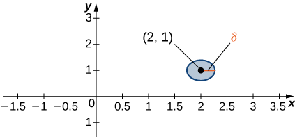
Consider a point \((a,b)∈\mathbb{R}^2.\) A \(δ\) disk centered at point \((a,b)\) is defined to be an open disk of radius \(δ\) centered at point \((a,b)\) —that is,
\[\{(x,y)∈\mathbb{R}^2∣(x−a)^2+(y−b)^2<δ^2\} \nonumber \]
as shown in Figure \(\PageIndex{1}\).
The idea of a \(δ\) disk appears in the definition of the limit of a function of two variables. If \(δ\) is small, then all the points \((x,y)\) in the \(δ\) disk are close to \((a,b)\). This is completely analogous to x being close to a in the definition of a limit of a function of one variable. In one dimension, we express this restriction as
\[a−δ<x<a+δ. \nonumber \]
In more than one dimension, we use a \(δ\) disk.
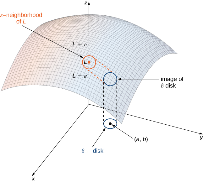
Let \(f\) be a function of two variables, \(x\) and \(y\). The limit of \(f(x,y)\) as \((x,y)\) approaches \((a,b)\) is \(L\), written
\[\lim_{(x,y)→(a,b)}f(x,y)=L \nonumber \]
if for each \(ε>0\) there exists a small enough \(δ>0\) such that for all points \((x,y)\) in a \(δ\) disk around \((a,b)\), except possibly for \((a,b)\) itself, the value of \(f(x,y)\) is no more than \(ε\) away from \(L\) (Figure \(\PageIndex{2}\)).
Using symbols, we write the following: For any \(ε>0\), there exists a number \(δ>0\) such that
\[|f(x,y)−L|<ε \nonumber \]
whenever
\[0<\sqrt{(x−a)^2+(y−b)^2}<δ. \nonumber \]
Proving that a limit exists using the definition of a limit of a function of two variables can be challenging. Instead, we use the following theorem, which gives us shortcuts to finding limits. The formulas in this theorem are an extension of the formulas in the limit laws theorem in The Limit Laws.
Let \(f(x,y)\) and \(g(x,y)\) be defined for all \((x,y)≠(a,b)\) in a neighborhood around \((a,b)\), and assume the neighborhood is contained completely inside the domain of \(f\). Assume that \(L\) and \(M\) are real numbers such that
\[\lim_{(x,y)→(a,b)}f(x,y)=L \nonumber \]
and
\[\lim_{(x,y)→(a,b)}g(x,y)=M, \nonumber \]
and let \(c\) be a constant. Then each of the following statements holds:
Constant Law:
\[\lim_{(x,y)→(a,b)}c=c \nonumber \]
Identity Laws:
\[\lim_{(x,y)→(a,b)}x=a \nonumber \]
\[\lim_{(x,y)→(a,b)}y=b \nonumber \]
Sum Law:
\[\lim_{(x,y)→(a,b)}(f(x,y)+g(x,y))=L+M \nonumber \]
Difference Law:
\[\lim_{(x,y)→(a,b)}(f(x,y)−g(x,y))=L−M \nonumber \]
Constant Multiple Law:
\[\lim_{(x,y)→(a,b)}(cf(x,y))=cL \nonumber \]
Product Law:
\[\lim_{(x,y)→(a,b)}(f(x,y)g(x,y))=LM \nonumber \]
Quotient Law:
\[\lim_{(x,y)→(a,b)}\dfrac{f(x,y)}{g(x,y)}=\dfrac{L}{M} \text{ for } M≠0 \nonumber \]
Power Law:
\[\lim_{(x,y)→(a,b)}(f(x,y))^n=L^n \nonumber \]
for any positive integer \(n\).
Root Law:
\[\lim_{(x,y)→(a,b)}\sqrt[n]{f(x,y)}=\sqrt[n]{L} \nonumber \]
for all \(L\) if \(n\) is odd and positive, and for \(L≥0\) if n is even and positive.
The proofs of these properties are similar to those for the limits of functions of one variable. We can apply these laws to finding limits of various functions.
Find each of the following limits:
- \(\displaystyle \lim_{(x,y)→(2,−1)}(x^2−2xy+3y^2−4x+3y−6)\)
- \(\displaystyle \lim_{(x,y)→(2,−1)}\dfrac{2x+3y}{4x−3y}\)
Solution
a. First use the sum and difference laws to separate the terms:
\[\begin{align*} \lim_{(x,y)→(2,−1)}(x^2−2xy+3y^2−4x+3y−6)\\ = \left(\lim_{(x,y)→(2,−1)}x^2 \right)− \left(\lim_{(x,y)→(2,−1)}2xy \right)+ \left(\lim_{(x,y)→(2,−1)}3y^2 \right)−\left(\lim_{(x,y)→(2,−1)}4x\right) \\ + \left(\lim_{(x,y)→(2,−1)}3y \right)−\left(\lim_{(x,y)→(2,−1)}6\right). \end{align*}\]
Next, use the constant multiple law on the second, third, fourth, and fifth limits:
\[\begin{align*} =(\lim_{(x,y)→(2,−1)}x^2)−2(\lim_{(x,y)→(2,−1)}xy)+3(\lim_{(x,y)→(2,−1)}y^2)−4(\lim_{(x,y)→(2,−1)}x) \\[4pt] +3(\lim_{(x,y)→(2,−1)}y)−\lim_{(x,y)→(2,−1)}6.\end{align*}\]
Now, use the power law on the first and third limits, and the product law on the second limit:
\[\begin{align*} \left(\lim_{(x,y)→(2,−1)}x\right)^2−2\left(\lim_{(x,y)→(2,−1)}x\right) \left(\lim_{(x,y)→(2,−1)}y\right)+3\left(\lim_{(x,y)→(2,−1)}y\right)^2 \\ −4\left(\lim_{(x,y)→(2,−1)}x\right)+3\left(\lim_{(x,y)→(2,−1)}y\right)−\lim_{(x,y)→(2,−1)}6. \end{align*}\]
Last, use the identity laws on the first six limits and the constant law on the last limit:
\[\begin{align*} \lim_{(x,y)→(2,−1)}(x^2−2xy+3y^2−4x+3y−6) = (2)^2−2(2)(−1)+3(−1)^2−4(2)+3(−1)−6 \\[4pt] =−6. \end{align*}\]
b. Before applying the quotient law, we need to verify that the limit of the denominator is nonzero. Using the difference law, constant multiple law, and identity law,
\[\begin{align*} \lim_{(x,y)→(2,−1)}(4x−3y) =\lim_{(x,y)→(2,−1)}4x−\lim_{(x,y)→(2,−1)}3y \\[4pt] =4(\lim_{(x,y)→(2,−1)}x)−3(\lim_{(x,y)→(2,−1)}y) \\[4pt] =4(2)−3(−1)=11. \end{align*}\]
Since the limit of the denominator is nonzero, the quotient law applies. We now calculate the limit of the numerator using the difference law, constant multiple law, and identity law:
\[\begin{align*} \lim_{(x,y)→(2,−1)}(2x+3y) =\lim_{(x,y)→(2,−1)}2x+\lim_{(x,y)→(2,−1)}3y \\[4pt] =2(\lim_{(x,y)→(2,−1)}x)+3(\lim_{(x,y)→(2,−1)}y) \\[4pt] =2(2)+3(−1)=1. \end{align*}\]
Therefore, according to the quotient law we have
\[\begin{align*} \lim_{(x,y)→(2,−1)}\dfrac{2x+3y}{4x−3y} =\dfrac{\displaystyle \lim_{(x,y)→(2,−1)}(2x+3y)}{\displaystyle \lim_{(x,y)→(2,−1)}(4x−3y)} \\[4pt] =\dfrac{1}{11}. \end{align*}\]
Evaluate the following limit:
\[\lim_{(x,y)→(5,−2)}\sqrt[3]{\dfrac{x^2−y}{y^2+x−1}}. \nonumber \]
- Hint
-
Use the limit laws.
- Answer
-
\[\displaystyle \lim_{(x,y)→(5,−2)}\sqrt[3]{\dfrac{x^2−y}{y^2+x−1}}=\dfrac{3}{2} \nonumber \]
Since we are taking the limit of a function of two variables, the point \((a,b)\) is in \(\mathbb{R}^2\), and it is possible to approach this point from an infinite number of directions. Sometimes when calculating a limit, the answer varies depending on the path taken toward \((a,b)\). If this is the case, then the limit fails to exist. In other words, the limit must be unique, regardless of path taken.
Show that neither of the following limits exist:
- \(\displaystyle \lim_{(x,y)→(0,0)}\dfrac{2xy}{3x^2+y^2}\)
- \(\displaystyle \lim_{(x,y)→(0,0)}\dfrac{4xy^2}{x^2+3y^4}\)
Solution
a. The domain of the function \(f(x,y)=\dfrac{2xy}{3x^2+y^2}\) consists of all points in the \(xy\)-plane except for the point \((0,0)\) (Figure \(\PageIndex{3}\)). To show that the limit does not exist as \((x,y)\) approaches \((0,0)\), we note that it is impossible to satisfy the definition of a limit of a function of two variables because of the fact that the function takes different values along different lines passing through point \((0,0)\). First, consider the line \(y=0\) in the \(xy\)-plane. Substituting \(y=0\) into \(f(x,y)\) gives
\[f(x,0)=\dfrac{2x(0)}{3x^2+0^2}=0 \nonumber \]
for any value of \(x\). Therefore the value of \(f\) remains constant for any point on the \(x\)-axis, and as \(y\) approaches zero, the function remains fixed at zero.
Next, consider the line \(y=x\). Substituting \(y=x\) into \(f(x,y)\) gives
\[f(x,x)=\dfrac{2x(x)}{3x^2+x^2}=\dfrac{2x^2}{4x^2}=\tfrac{1}{2}. \nonumber \]
This is true for any point on the line \(y=x\). If we let \(x\) approach zero while staying on this line, the value of the function remains fixed at \(\tfrac{1}{2}\), regardless of how small \(x\) is.
Choose a value for ε that is less than \(1/2\)—say, \(1/4\). Then, no matter how small a \(δ\) disk we draw around \((0,0)\), the values of \(f(x,y)\) for points inside that \(δ\) disk will include both \(0\) and \(\tfrac{1}{2}\). Therefore, the definition of limit at a point is never satisfied and the limit fails to exist.
b. In a similar fashion to a., we can approach the origin along any straight line passing through the origin. If we try the \(x\)-axis (i.e., \(y=0\)), then the function remains fixed at zero. The same is true for the \(y\)-axis. Suppose we approach the origin along a straight line of slope \(k\). The equation of this line is \(y=kx\). Then the limit becomes
\[\begin{align*} \lim_{(x,y)→(0,0)}\dfrac{4xy^2}{x^2+3y^4} = \lim_{(x,y)→(0,0)}\dfrac{4x(kx)^2}{x^2+3(kx)^4} \\ = \lim_{(x,y)→(0,0)}\dfrac{4k^2x^3}{x^2+3k^4x^4} \\ =\lim_{(x,y)→(0,0)}\dfrac{4k^2x}{1+3k^4x^2} \\ = \dfrac{\displaystyle \lim_{(x,y)→(0,0)}(4k^2x)}{\displaystyle \lim_{(x,y)→(0,0)}(1+3k^4x^2)} \\ = 0. \end{align*}\]
regardless of the value of \(k\). It would seem that the limit is equal to zero. What if we chose a curve passing through the origin instead? For example, we can consider the parabola given by the equation \(x=y^2\). Substituting \(y^2\) in place of \(x\) in \(f(x,y)\) gives
\[\begin{align*}\lim_{(x,y)→(0,0)}\dfrac{4xy^2}{x^2+3y^4} = \lim_{(x,y)→(0,0)}\dfrac{4(y^2)y^2}{(y^2)^2+3y^4} \\ = \lim_{(x,y)→(0,0)}\dfrac{4y^4}{y^4+3y^4} \\ = \lim_{(x,y)→(0,0)}1 \\ = 1. \end{align*}\]
By the same logic in part a, it is impossible to find a δ disk around the origin that satisfies the definition of the limit for any value of \(ε<1.\) Therefore,
\[\displaystyle \lim_{(x,y)→(0,0)}\dfrac{4xy^2}{x^2+3y^4} \nonumber \]
does not exist.
Show that
\[\lim_{(x,y)→(2,1)}\dfrac{(x−2)(y−1)}{(x−2)^2+(y−1)^2} \nonumber \]
does not exist.
- Hint
-
Pick a line with slope \(k\) passing through point \((2,1).\)
- Answer
-
If \(y=k(x−2)+1,\) then \(\lim_{(x,y)→(2,1)}\dfrac{(x−2)(y−1)}{(x−2)^2+(y−1)^2}=\dfrac{k}{1+k^2}\). Since the answer depends on \(k,\) the limit fails to exist.
Interior Points and Boundary Points
To study continuity and differentiability of a function of two or more variables, we first need to learn some new terminology.
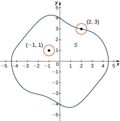
Let \(S\) be a subset of \(\mathbb{R}^2\) (Figure \(\PageIndex{4}\)).
- A point \(P_0\) is called an interior point of \(S\) if there is a \(δ\) disk centered around \(P_0\) contained completely in \(S\).
- A point \(P_0\) is called a boundary point of \(S\) if every \(δ\) disk centered around \(P_0\) contains points both inside and outside \(S\).
Let \(S\) be a subset of \(\mathbb{R}^2\) (Figure \(\PageIndex{4}\)).
- \(S\) is called an open set if every point of \(S\) is an interior point.
- \(S\) is called a closed set if it contains all its boundary points.
An example of an open set is a \(δ\) disk. If we include the boundary of the disk, then it becomes a closed set. A set that contains some, but not all, of its boundary points is neither open nor closed. For example if we include half the boundary of a \(δ\) disk but not the other half, then the set is neither open nor closed.
Let \(S\) be a subset of \(\mathbb{R}^2\) (Figure \(\PageIndex{4}\)).
- An open set \(S\) is a connected set if it cannot be represented as the union of two or more disjoint, nonempty open subsets.
- A set \(S\) is a region if it is open, connected, and nonempty.
The definition of a limit of a function of two variables requires the \(δ\) disk to be contained inside the domain of the function. However, if we wish to find the limit of a function at a boundary point of the domain, the \(δ\) disk is not contained inside the domain. By definition, some of the points of the \(δ\) disk are inside the domain and some are outside. Therefore, we need only consider points that are inside both the \(δ\) disk and the domain of the function. This leads to the definition of the limit of a function at a boundary point.
Let \(f\) be a function of two variables, \(x\) and \(y\), and suppose \((a,b)\) is on the boundary of the domain of \(f\). Then, the limit of \(f(x,y)\) as \((x,y)\) approaches \((a,b)\) is \(L\), written
\[\lim_{(x,y)→(a,b)}f(x,y)=L, \nonumber \]
if for any \(ε>0,\) there exists a number \(δ>0\) such that for any point \((x,y)\) inside the domain of \(f\) and within a suitably small distance positive \(δ\) of \((a,b),\) the value of \(f(x,y)\) is no more than \(ε\) away from \(L\) (Figure \(\PageIndex{2}\)). Using symbols, we can write: For any \(ε>0\), there exists a number \(δ>0\) such that
\[|f(x,y)−L|<ε\, \text{whenever}\, 0<\sqrt{(x−a)^2+(y−b)^2}<δ. \nonumber \]
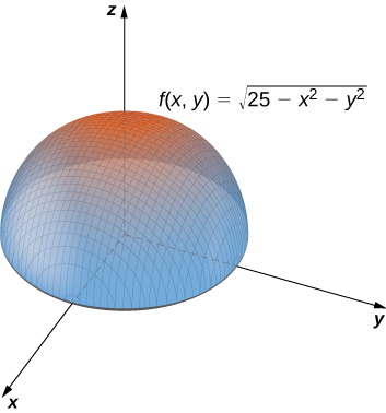
Prove
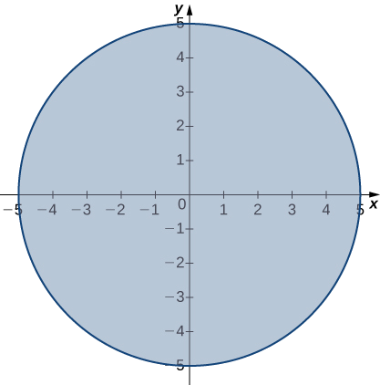
\[\lim_{(x,y)→(4,3)}\sqrt{25−x^2−y^2}=0. \nonumber \]
Solution
The domain of the function \(f(x,y)=\sqrt{25−x^2−y^2}\) is \(\big\{(x,y)∈\mathbb{R}^2∣x^2+y^2≤25\big\}\), which is a circle of radius \(5\) centered at the origin, along with its interior as shown in Figure \(\PageIndex{5}\).
We can use the limit laws, which apply to limits at the boundary of domains as well as interior points:
\[\begin{align*} \lim_{(x,y)→(4,3)}\sqrt{25−x^2−y^2} =\sqrt{\lim_{(x,y)→(4,3)}(25−x^2−y^2)} \\ = \sqrt{\lim_{(x,y)→(4,3)}25−\lim_{(x,y)→(4,3)}x^2−\lim_{(x,y)→(4,3)}y^2} \\ =\sqrt{25−4^2−3^2} \\ = 0 \end{align*}\]
See the following graph.
Evaluate the following limit:
\[\lim_{(x,y)→(5,−2)}\sqrt{29−x^2−y^2}. \nonumber \]
- Hint
-
Determine the domain of \(f(x,y)=\sqrt{29−x^2−y^2}\).
- Answer
-
\[\lim_{(x,y)→(5,−2)}\sqrt{29−x^2−y^2} \nonumber \]
Continuity of Functions of Two Variables
In Continuity, we defined the continuity of a function of one variable and saw how it relied on the limit of a function of one variable. In particular, three conditions are necessary for \(f(x)\) to be continuous at point \(x=a\)
- \(f(a)\) exists.
- \(\displaystyle \lim_{x→a}f(x)\) exists.
- \(\displaystyle \lim_{x→a}f(x)=f(a).\)
These three conditions are necessary for continuity of a function of two variables as well.
A function \(f(x,y)\) is continuous at a point \((a,b)\) in its domain if the following conditions are satisfied:
- \(f(a,b)\) exists.
- \(\displaystyle \lim_{(x,y)→(a,b)}f(x,y)\) exists.
- \(\displaystyle \lim_{(x,y)→(a,b)}f(x,y)=f(a,b).\)
Show that the function
\[f(x,y)=\dfrac{3x+2y}{x+y+1} \nonumber \]
is continuous at point \((5,−3).\)
Solution
There are three conditions to be satisfied, per the definition of continuity. In this example, \(a=5\) and \(b=−3.\)
1. \(f(a,b)\) exists. This is true because the domain of the function f consists of those ordered pairs for which the denominator is nonzero (i.e., \(x+y+1≠0\)). Point \((5,−3)\) satisfies this condition. Furthermore,
\[f(a,b)=f(5,−3)=\dfrac{3(5)+2(−3)}{5+(−3)+1}=\dfrac{15−6}{2+1}=3. \nonumber \]
2. \(\displaystyle \lim_{(x,y)→(a,b)}f(x,y)\) exists. This is also true:
\[\begin{align*} \lim_{(x,y)→(a,b)}f(x,y) =\lim_{(x,y)→(5,−3)}\dfrac{3x+2y}{x+y+1} \\ =\dfrac{\displaystyle \lim_{(x,y)→(5,−3)}(3x+2y)}{\displaystyle \lim_{(x,y)→(5,−3)}(x+y+1)} \\ = \dfrac{15−6}{5−3+1} \\ = 3. \end{align*}\]
3. \(\displaystyle \lim_{(x,y)→(a,b)}f(x,y)=f(a,b).\) This is true because we have just shown that both sides of this equation equal three.
Show that the function
\[f(x,y)=\sqrt{26−2x^2−y^2}\nonumber \]
is continuous at point \((2,−3)\).
- Hint
-
Use the three-part definition of continuity.
- Answer
-
- The domain of \(f\) contains the ordered pair \((2,−3)\) because \(f(a,b)=f(2,−3)=\sqrt{16−2(2)^2−(−3)^2}=3\)
- \(\displaystyle \lim_{(x,y)→(a,b)}f(x,y)=3\)
- \(\displaystyle \lim_{(x,y)→(a,b)}f(x,y)=f(a,b)=3\)
Continuity of a function of any number of variables can also be defined in terms of delta and epsilon. A function of two variables is continuous at a point \((x_0,y_0)\) in its domain if for every \(ε>0\) there exists a \(δ>0\) such that, whenever \(\sqrt{(x−x_0)^2+(y−y_0)^2}<δ\) it is true, \(|f(x,y)−f(a,b)|<ε.\) This definition can be combined with the formal definition (that is, the epsilon–delta definition) of continuity of a function of one variable to prove the following theorems:
If \(f(x,y)\) is continuous at \((x_0,y_0)\), and \(g(x,y)\) is continuous at \((x_0,y_0)\), then \(f(x,y)+g(x,y)\) is continuous at \((x_0,y_0)\).
If \(g(x)\) is continuous at \(x_0\) and \(h(y)\) is continuous at \(y_0\), then \(f(x,y)=g(x)h(y)\) is continuous at \((x_0,y_0).\)
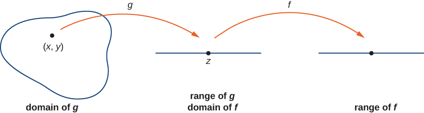
Let \(g\) be a function of two variables from a domain \(D⊆\mathbb{R}^2\) to a range \(R⊆R.\) Suppose \(g\) is continuous at some point \((x_0,y_0)∈D\) and define \(z_0=g(x_0,y_0)\). Let f be a function that maps \(R\) to \(R\) such that \(z_0\) is in the domain of \(f\). Last, assume \(f\) is continuous at \(z_0\). Then \(f∘g\) is continuous at \((x_0,y_0)\) as shown in Figure \(\PageIndex{7}\).
Let’s now use the previous theorems to show continuity of functions in the following examples.
Show that the functions \(f(x,y)=4x^3y^2\) and \(g(x,y)=\cos(4x^3y^2)\) are continuous everywhere.
Solution
The polynomials \(g(x)=4x^3\) and \(h(y)=y^2\) are continuous at every real number, and therefore by the product of continuous functions theorem, \(f(x,y)=4x^3y^2\) is continuous at every point \((x,y)\) in the \(xy\)-plane. Since \(f(x,y)=4x^3y^2\) is continuous at every point \((x,y)\) in the \(xy\)-plane and \(g(x)=\cos x\) is continuous at every real number \(x\), the continuity of the composition of functions tells us that \(g(x,y)=\cos(4x^3y^2)\) is continuous at every point \((x,y)\) in the \(xy\)-plane.
Show that the functions \(f(x,y)=2x^2y^3+3\) and \(g(x,y)=(2x^2y^3+3)^4\) are continuous everywhere.
- Hint
-
Use the continuity of the sum, product, and composition of two functions.
- Answer
-
The polynomials \(g(x)=2x^2\) and \(h(y)=y^3\) are continuous at every real number; therefore, by the product of continuous functions theorem, \(f(x,y)=2x^2y^3\) is continuous at every point \((x,y)\) in the \(xy\)-plane. Furthermore, any constant function is continuous everywhere, so \(g(x,y)=3\) is continuous at every point \((x,y)\) in the \(xy\)-plane. Therefore, \(f(x,y)=2x^2y^3+3\) is continuous at every point \((x,y)\) in the \(xy\)-plane. Last, \(h(x)=x^4\) is continuous at every real number \(x\), so by the continuity of composite functions theorem \(g(x,y)=(2x^2y^3+3)^4\) is continuous at every point \((x,y)\) in the \(xy\)-plane.
Functions of Three or More Variables
The limit of a function of three or more variables occurs readily in applications. For example, suppose we have a function \(f(x,y,z)\) that gives the temperature at a physical location \((x,y,z)\) in three dimensions. Or perhaps a function \(g(x,y,z,t)\) can indicate air pressure at a location \((x,y,z)\) at time \(t\). How can we take a limit at a point in \(\mathbb{R}^3\)? What does it mean to be continuous at a point in four dimensions?
The answers to these questions rely on extending the concept of a \(δ\) disk into more than two dimensions. Then, the ideas of the limit of a function of three or more variables and the continuity of a function of three or more variables are very similar to the definitions given earlier for a function of two variables.
Let \((x_0,y_0,z_0)\) be a point in \(\mathbb{R}^3\). Then, a \(δ\)-ball in three dimensions consists of all points in \(\mathbb{R}^3\) lying at a distance of less than \(δ\) from \((x_0,y_0,z_0)\) —that is,
\[\big\{(x,y,z)∈\mathbb{R}^3∣\sqrt{(x−x_0)^2+(y−y_0)^2+(z−z_0)^2}<δ\big\}. \nonumber \]
To define a \(δ\)-ball in higher dimensions, add additional terms under the radical to correspond to each additional dimension. For example, given a point \(P=(w_0,x_0,y_0,z_0)\) in \(\mathbb{R}^4\), a \(δ\) ball around \(P\) can be described by
\[\big\{(w,x,y,z)∈\mathbb{R}^4∣\sqrt{(w−w_0)^2+(x−x_0)^2+(y−y_0)^2+(z−z_0)^2}<δ\big\}. \nonumber \]
To show that a limit of a function of three variables exists at a point \((x_0,y_0,z_0)\), it suffices to show that for any point in a \(δ\) ball centered at \((x_0,y_0,z_0)\), the value of the function at that point is arbitrarily close to a fixed value (the limit value). All the limit laws for functions of two variables hold for functions of more than two variables as well.
Find
\[\lim_{(x,y,z)→(4,1,−3)}\dfrac{x^2y−3z}{2x+5y−z}. \nonumber \]
Solution
Before we can apply the quotient law, we need to verify that the limit of the denominator is nonzero. Using the difference law, the identity law, and the constant law,
\[\begin{align*}\lim_{(x,y,z)→(4,1,−3)}(2x+5y−z) =2(\lim_{(x,y,z)→(4,1,−3)}x)+5(\lim_{(x,y,z)→(4,1,−3)}y)−(\lim_{(x,y,z)→(4,1,−3)}z) \\ = 2(4)+5(1)−(−3) \\ = 16. \end{align*}\]
Since this is nonzero, we next find the limit of the numerator. Using the product law, power law, difference law, constant multiple law, and identity law,
\[\begin{align*} \lim_{(x,y,z)→(4,1,−3)}(x^2y−3z) =(\lim_{(x,y,z)→(4,1,−3)}x)^2(\lim_{(x,y,z)→(4,1,−3)}y)−3\lim_{(x,y,z)→(4,1,−3)}z \\ =(4^2)(1)−3(−3) \\ = 16+9 \\ = 25 \end{align*}\]
Last, applying the quotient law:
\[\lim_{(x,y,z)→(4,1,−3)}\dfrac{x^2y−3z}{2x+5y−z}=\dfrac{\displaystyle \lim_{(x,y,z)→(4,1,−3)}(x^2y−3z)}{\displaystyle \lim_{(x,y,z)→(4,1,−3)}(2x+5y−z)}=\dfrac{25}{16} \nonumber \]
Find
\[\lim_{(x,y,z)→(4,−1,3)}\sqrt{13−x^2−2y^2+z^2} \nonumber \]
- Hint
-
Use the limit laws and the continuity of the composition of functions.
- Answer
-
\[\lim_{(x,y,z)→(4,−1,3)}\sqrt{13−x^2−2y^2+z^2}=2 \nonumber \]
Key Concepts
- To study limits and continuity for functions of two variables, we use a \(δ\) disk centered around a given point.
- A function of several variables has a limit if for any point in a \(δ\) ball centered at a point \(P\), the value of the function at that point is arbitrarily close to a fixed value (the limit value).
- The limit laws established for a function of one variable have natural extensions to functions of more than one variable.
- A function of two variables is continuous at a point if the limit exists at that point, the function exists at that point, and the limit and function are equal at that point.
Glossary
- boundary point
- a point \(P_0\) of \(R\) is a boundary point if every \(δ\) disk centered around \(P_0\) contains points both inside and outside \(R\)
- closed set
- a set \(S\) that contains all its boundary points
- connected set
- an open set \(S\) that cannot be represented as the union of two or more disjoint, nonempty open subsets
- \(δ\) disk
- an open disk of radius \(δ\) centered at point \((a,b)\)
- \(δ\) ball
- all points in \(\mathbb{R}^3\) lying at a distance of less than \(δ\) from \((x_0,y_0,z_0)\)
- interior point
- a point \(P_0\) of \(\mathbb{R}\) is a boundary point if there is a \(δ\) disk centered around \(P_0\) contained completely in \(\mathbb{R}\)
- open set
- a set \(S\) that contains none of its boundary points
- region
- an open, connected, nonempty subset of \(\mathbb{R}^2\)