
2.4: Bifurcations
- Page ID
- 122443

\( \newcommand{\vecs}[1]{\overset { \scriptstyle \rightharpoonup} {\mathbf{#1}} } \)
\( \newcommand{\vecd}[1]{\overset{-\!-\!\rightharpoonup}{\vphantom{a}\smash {#1}}} \)
\( \newcommand{\dsum}{\displaystyle\sum\limits} \)
\( \newcommand{\dint}{\displaystyle\int\limits} \)
\( \newcommand{\dlim}{\displaystyle\lim\limits} \)
\( \newcommand{\id}{\mathrm{id}}\) \( \newcommand{\Span}{\mathrm{span}}\)
( \newcommand{\kernel}{\mathrm{null}\,}\) \( \newcommand{\range}{\mathrm{range}\,}\)
\( \newcommand{\RealPart}{\mathrm{Re}}\) \( \newcommand{\ImaginaryPart}{\mathrm{Im}}\)
\( \newcommand{\Argument}{\mathrm{Arg}}\) \( \newcommand{\norm}[1]{\| #1 \|}\)
\( \newcommand{\inner}[2]{\langle #1, #2 \rangle}\)
\( \newcommand{\Span}{\mathrm{span}}\)
\( \newcommand{\id}{\mathrm{id}}\)
\( \newcommand{\Span}{\mathrm{span}}\)
\( \newcommand{\kernel}{\mathrm{null}\,}\)
\( \newcommand{\range}{\mathrm{range}\,}\)
\( \newcommand{\RealPart}{\mathrm{Re}}\)
\( \newcommand{\ImaginaryPart}{\mathrm{Im}}\)
\( \newcommand{\Argument}{\mathrm{Arg}}\)
\( \newcommand{\norm}[1]{\| #1 \|}\)
\( \newcommand{\inner}[2]{\langle #1, #2 \rangle}\)
\( \newcommand{\Span}{\mathrm{span}}\) \( \newcommand{\AA}{\unicode[.8,0]{x212B}}\)
\( \newcommand{\vectorA}[1]{\vec{#1}} % arrow\)
\( \newcommand{\vectorAt}[1]{\vec{\text{#1}}} % arrow\)
\( \newcommand{\vectorB}[1]{\overset { \scriptstyle \rightharpoonup} {\mathbf{#1}} } \)
\( \newcommand{\vectorC}[1]{\textbf{#1}} \)
\( \newcommand{\vectorD}[1]{\overrightarrow{#1}} \)
\( \newcommand{\vectorDt}[1]{\overrightarrow{\text{#1}}} \)
\( \newcommand{\vectE}[1]{\overset{-\!-\!\rightharpoonup}{\vphantom{a}\smash{\mathbf {#1}}}} \)
\( \newcommand{\vecs}[1]{\overset { \scriptstyle \rightharpoonup} {\mathbf{#1}} } \)
\(\newcommand{\longvect}{\overrightarrow}\)
\( \newcommand{\vecd}[1]{\overset{-\!-\!\rightharpoonup}{\vphantom{a}\smash {#1}}} \)
\(\newcommand{\avec}{\mathbf a}\) \(\newcommand{\bvec}{\mathbf b}\) \(\newcommand{\cvec}{\mathbf c}\) \(\newcommand{\dvec}{\mathbf d}\) \(\newcommand{\dtil}{\widetilde{\mathbf d}}\) \(\newcommand{\evec}{\mathbf e}\) \(\newcommand{\fvec}{\mathbf f}\) \(\newcommand{\nvec}{\mathbf n}\) \(\newcommand{\pvec}{\mathbf p}\) \(\newcommand{\qvec}{\mathbf q}\) \(\newcommand{\svec}{\mathbf s}\) \(\newcommand{\tvec}{\mathbf t}\) \(\newcommand{\uvec}{\mathbf u}\) \(\newcommand{\vvec}{\mathbf v}\) \(\newcommand{\wvec}{\mathbf w}\) \(\newcommand{\xvec}{\mathbf x}\) \(\newcommand{\yvec}{\mathbf y}\) \(\newcommand{\zvec}{\mathbf z}\) \(\newcommand{\rvec}{\mathbf r}\) \(\newcommand{\mvec}{\mathbf m}\) \(\newcommand{\zerovec}{\mathbf 0}\) \(\newcommand{\onevec}{\mathbf 1}\) \(\newcommand{\real}{\mathbb R}\) \(\newcommand{\twovec}[2]{\left[\begin{array}{r}#1 \\ #2 \end{array}\right]}\) \(\newcommand{\ctwovec}[2]{\left[\begin{array}{c}#1 \\ #2 \end{array}\right]}\) \(\newcommand{\threevec}[3]{\left[\begin{array}{r}#1 \\ #2 \\ #3 \end{array}\right]}\) \(\newcommand{\cthreevec}[3]{\left[\begin{array}{c}#1 \\ #2 \\ #3 \end{array}\right]}\) \(\newcommand{\fourvec}[4]{\left[\begin{array}{r}#1 \\ #2 \\ #3 \\ #4 \end{array}\right]}\) \(\newcommand{\cfourvec}[4]{\left[\begin{array}{c}#1 \\ #2 \\ #3 \\ #4 \end{array}\right]}\) \(\newcommand{\fivevec}[5]{\left[\begin{array}{r}#1 \\ #2 \\ #3 \\ #4 \\ #5 \\ \end{array}\right]}\) \(\newcommand{\cfivevec}[5]{\left[\begin{array}{c}#1 \\ #2 \\ #3 \\ #4 \\ #5 \\ \end{array}\right]}\) \(\newcommand{\mattwo}[4]{\left[\begin{array}{rr}#1 \amp #2 \\ #3 \amp #4 \\ \end{array}\right]}\) \(\newcommand{\laspan}[1]{\text{Span}\{#1\}}\) \(\newcommand{\bcal}{\cal B}\) \(\newcommand{\ccal}{\cal C}\) \(\newcommand{\scal}{\cal S}\) \(\newcommand{\wcal}{\cal W}\) \(\newcommand{\ecal}{\cal E}\) \(\newcommand{\coords}[2]{\left\{#1\right\}_{#2}}\) \(\newcommand{\gray}[1]{\color{gray}{#1}}\) \(\newcommand{\lgray}[1]{\color{lightgray}{#1}}\) \(\newcommand{\rank}{\operatorname{rank}}\) \(\newcommand{\row}{\text{Row}}\) \(\newcommand{\col}{\text{Col}}\) \(\renewcommand{\row}{\text{Row}}\) \(\newcommand{\nul}{\text{Nul}}\) \(\newcommand{\var}{\text{Var}}\) \(\newcommand{\corr}{\text{corr}}\) \(\newcommand{\len}[1]{\left|#1\right|}\) \(\newcommand{\bbar}{\overline{\bvec}}\) \(\newcommand{\bhat}{\widehat{\bvec}}\) \(\newcommand{\bperp}{\bvec^\perp}\) \(\newcommand{\xhat}{\widehat{\xvec}}\) \(\newcommand{\vhat}{\widehat{\vvec}}\) \(\newcommand{\uhat}{\widehat{\uvec}}\) \(\newcommand{\what}{\widehat{\wvec}}\) \(\newcommand{\Sighat}{\widehat{\Sigma}}\) \(\newcommand{\lt}{<}\) \(\newcommand{\gt}{>}\) \(\newcommand{\amp}{&}\) \(\definecolor{fillinmathshade}{gray}{0.9}\)In many models of real-life situations (e.g., population models, pollution models, etc.), it is useful to use parameters in addition to the variables involved. A parameter is a quantity (usually denoted by a letter) whose value does not depend on the value of the independent variable (often time) but represents a characteristic of the situation being modeled. For example, in the differential equation for the exponential model for population growth
\[\dfrac{dP}{dt} = kP, \nonumber\]
there is a parameter \(k\). Here \(k\) is the constant of proportionality for the population's growth rate. Depending on the species we're modeling, we would expect the value of this proportionality constant \(k\) to be different. It is a characteristic of the species being modeled.
In other differential equation models, the values of the parameters may be much more flexible and can vary greatly, depending on other factors in the situation. For example, a certain fish population has the following exponential growth differential equation:
\[\dfrac{dP}{dt} = 0.2P. \nonumber\]
If we set an annual fishing quota \(q\) (total fish of this species caught by fishing boats each year) the population's growth rate may be modeled by the following differential equation:
\[\dfrac{dP}{dt} = 0.2P - q \nonumber\]
Here \(q\) is a parameter representing the number of fish of this species that are caught each year. This time the parameter is not a characteristic of the fish species, but is a value that we can choose to vary in our model (although this would be challenging to control precisely in real-life).
In this section, we will focus on these parameters, looking for changes in the behavior of the solutions of a differential equation as its parameters are varied. Most of the time, small changes in one of these parameters results in small changes in the behavior of the solution curves. But sometimes, a small change in a parameter can cause the long-term behavior of the solutions to become drastically different. This drastic change is typically a change in the number of equilibrium solutions present or a change in the type of stability of one or more of the equilibrium solutions. A differential equation with one equilibrium solution may suddenly have two equilibrium solutions. Or a differential equation with two equilibrium solutions may suddenly have only one equilibrium solution or none. Or the single stable equilibrium of a differential equation may suddenly become an unstable equilibrium. A drastic change of this sort (typically a change in the number of equilibrium solutions or a change in the type of stability of an equilibrium) is called a bifurcation.
The value of the parameter where a bifurcation occurs is called a bifucation point.
Consider the differential equation \[ \dfrac{dP}{dt} = 0.2P - q \nonumber \]
Note that adjusting the value of \(q\) on its viable range \([0, \infty)\) only shifts the equilibrium solution up and down to the current horizontal line given by \(y = 5q\). And observe that in each case, this equilibrium will be an unstable equilibrium. Since this ODE (ordinary differential equation) always has a single unstable equilibrium solution for every value of \(q,\) with no change in the number of equilibrium solutions or in the nature of the equilibrium (the type of stability), this differential equation does not have a bifurcation.
Detecting Bifurcations in a Differential Equation with a Parameter
Now let's consider a differential equation with a parameter where a bifurcation does occur.
Consider the differential equation with parameter \(a\),
\[\dfrac{dy}{dt}=y^2 + 2y + a \nonumber\]
Determine whether this differential equation has a bifurcation point or multiple bifurcation points and identify them.
Solution
Trial-and-Error Approach:
As a way to explore this problem more concretely, let's start by using a trial-and-error approach to look for a bifurcation.
We'll select several convenient values of the parameter \(a\) that will make the resulting ODE easy to factor and identify the corresponding equilibrium solution(s). This may not always be easy to do, but it's not very difficult in this example.
Trial 1: Let \(a = 0.\) This is often a nice value to start with.
Then \[\dfrac{dy}{dt}=y^2 + 2y \nonumber\]
Solving for the equilibrium solution(s), we set the ODE equal to \(0\), factor and solve for \(y.\)
\[\begin{align*} y^2 + 2y &= 0 \\[4pt]
y(y+2) &= 0 \end{align*}\]
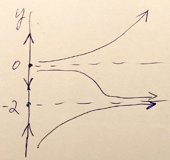
So \(y = -2\) and \(y = 0\) are critical numbers of this ODE and correspond to two equilibrium solutions of the ODE.
To create a phase line for this ODE, we first draw (and label) the vertical \(y\)-axis, label the critical points on this axis and then sketch in the corresponding equilibrium solutions with dashed lines.
Next, we will need to check the sign of \(\dfrac{dy}{dt}\) for a value of \(y\) below \(-2\), for a value between \(-2\) and \(0\) and for a value greater than \(0.\) To make it easier to evaluate, we'll choose to evaluate the factored form of \(\dfrac{dy}{dt}.\)
\[\begin{align*} \text{At }y = -3, \quad \dfrac{dy}{dt} \Bigg|_{y \,=\, -3} &= -3(-3 + 2) = 3 > 0. & & \text{So solutions will be increasing for }y <-2.\\[5pt]
\text{At }y = -1, \quad \dfrac{dy}{dt} \Bigg|_{y\,=\, -1} &= -1(-1 + 2) = -1 < 0. & & \text{So solutions will be decreasing between }y=-2\text{ and }y=0.\\[5pt]
\text{At }y = 1, \quad \dfrac{dy}{dt} \Bigg|_{y \,=\, 1} &= 1(1 + 2) = 3 > 0. & & \text{So solutions will be increasing for }y>0.\end{align*} \]
This gives us the following phase line with corresponding representative solution curves.
Trial 2: Let \(a = 1.\)
Here we aren't just picking the next nice number, but rather, we're considering what would be the next nice value for a so that the resulting polynomial is easy to factor.
Here we get the ODE \[\dfrac{dy}{dt}=y^2 + 2y +1\nonumber\]
Solving for the critical numbers/equilibrium solution(s), we set the ODE equal to \(0\), factor and solve for \(y.\)
\[\begin{align*} y^2 + 2y + 1&= 0 \\[4pt]
(y+1)^2 &= 0 \end{align*}\]
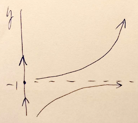
So \(y = -1\) is a repeated solution and thus is the only equilibrium solution of this ODE. Since we see that we have only one equilibrium when \(a = 1,\) we know that this ODE (with parameter \(a\)) has a bifurcation point, since we saw a change in the number of equilibrium solutions when we changed the value of \(a.\) Now this does not guarantee that the value \(a = 1\) is the bifurcation point, since we don't yet know if it is really the boundary value where the number of equilibrium solutions changed from two to one.
Once we've considered the graphical approach below, it will be easier to see that the value \(a = 1\) is indeed a bifurcation point, since it is the value for which we get a perfect square trinomial for \(\dfrac{dy}{dt}\) and a repeated solution when we set \(\dfrac{dy}{dt}\) equal to \(0.\) There is actually no other value of \(a\) for which this ODE will have a single equilibrium solution.
Now let's create a phase line for this ODE with a single equilibrium solution. Again we start by drawing (and labeling) the vertical \(y\)-axis, place our critical point and sketch the corresponding equilibrium solution as a dashed line.
Then we check the sign of \(\dfrac{dy}{dt}\) for a value of \(y\) below \(-1\) and for a value greater than \(-1.\) To make it easier to evaluate, we'll again choose to evaluate the factored form of \(\dfrac{dy}{dt}.\)
\[\begin{align*} \text{At }y = -2, \quad \dfrac{dy}{dt} \Bigg|_{y \,=\, -2} &= (-2 + 1)^2 = 1 > 0. & & \text{So solutions will be increasing for }y<-1.\\[5pt]
\text{At }y = 0, \quad \dfrac{dy}{dt} \Bigg|_{y\,=\, 0} &= (0 + 1)^2 = 1 > 0. & & \text{So solutions will also be increasing for }y>-1.\end{align*} \]
This gives us the following phase line with corresponding representative solution curves.
Trial 3: Let \(a = 2.\)
Here we really are just picking the next nice number, since, if you consider this polynomial carefully, you'll see that with middle term "\(+2y,\)" we won't be able to find any positive value for \(a\) larger than \(1\) that will result in a trinomial we can factor.
So this time we end up with the ODE \[\dfrac{dy}{dt}=y^2 + 2y +2\nonumber\]
Solving for the equilibrium solution(s), we set the ODE equal to \(0\) and solve for \(y.\) This time, since it does not factor, we use the quadratic formula.
\[\begin{align*} y^2 + 2y + 2&= 0 \\[5pt]
y &= \dfrac{-2 \pm \sqrt{4 - 4(1)(2)}}{2} = \dfrac{-2 \pm \sqrt{-4}}{2} \\[5pt]
&= -1 \pm i \end{align*}\]
We end up with two complex imaginary solutions. Since values of the dependent variable need to be real numbers in this problem, this means that this ODE has no equilibrium solutions. So we went from two equilibrium solutions for \(a = 0\) to one equilibrium solution when \(a = 1\) and now no equilibrium solutions for \(a = 2.\) If we were to try any other values of \(a\) greater than \(1,\) we would also find no equilibrium solutions. And if we try any other values of \(a\) less than \(1,\) we'll obtain two corresponding equilibrium solutions. We'll actually do this as part of our work for Example \(\PageIndex{4}\) below.
Putting these results together allows us to conclude with confidence that this differential equation with parameter \(a\)
\[\dfrac{dy}{dt}=y^2 + 2y + a \nonumber\]
has a single bifurcation at the bifurcation point \(a = 1.\)
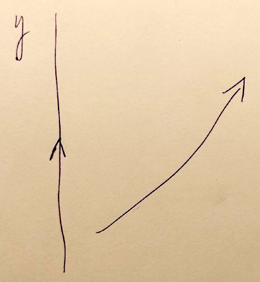
For the sake of completion, and to prepare us for the next step later in this section, let's create the phase line for this third ODE with no equilibrium solutions. Start by drawing (and labeling) the vertical \(y\)-axis. Since there are no critical points, we go on to the next step.
We will need to check the sign of \(\dfrac{dy}{dt}\) for any value of \(y\) (since we found no equilibrium solutions).
\[\begin{align*} \text{At }y = 0, \quad \dfrac{dy}{dt} \Bigg|_{y \,=\, 0} &= (0)^2 +2(0) + 2 = 2 > 0. & & \text{So solutions will be increasing everywhere.}\end{align*} \]
This gives us the following phase line with corresponding representative solution curves.
Looking for a Better Way to Identify Bifurcations
Although we were able to determine the bifurcation point for this differential equation by trying out a few values of the parameter \(a,\) bifurcation points are not usually so easy to find in this way. Below we will discuss two additional methods we can use to determine if a given differential equation with a parameter has a bifurcation or not.
As we did above in the Trial-and-Error approach, we usually consider the zeros of the function
\[ f(y) = \dfrac{dy}{dt} \nonumber\]
to help us determine whether a given differential equation has a bifurcation.
That is, we're looking for the equilibrium solutions of the ODE in terms of the parameter, in order to consider if the number of these equilibrium solutions changes as the parameter varies.
Using this thinking, let's consider two additional ways we can look for bifurcation points: algebraically and graphically. In Examples \(\PageIndex{2}\) and \(\PageIndex{3}\), we'll demonstrate these methods to explore the same ODE we examined in Example \(\PageIndex{1}\) above.
Consider again the differential equation from Example \(\PageIndex{1}\) with parameter \(a\),
\[\dfrac{dy}{dt}=y^2 + 2y + a \nonumber\]
Use an algebraic approach to determine whether this differential equation has a bifurcation point or multiple bifurcation points and identify them.
Solution
Algebraic Approach:
We'll start by setting \(f(y) = 0\) and solve for \(y\) in terms of the parameter \(a\). If this formula allows us to obtain a different number of equilibrium solutions depending on the value of \(a\), then we will find at least one bifurcation point.
\[y^2 + 2y + a = 0 \nonumber\]
Solving this equation for \(y,\) we obtain
\[\begin{align*} y &= \dfrac{-2 \pm \sqrt{4 - 4(1)(a)}}{2} \\[5pt]
&= \dfrac{-2}{2} \pm \dfrac{\sqrt{4 - 4a}}{2} \\[5pt]
&= -1 \pm \dfrac{2\sqrt{1 - a}}{2} \\[5pt]
&= -1 \pm \sqrt{1 - a} \end{align*}\]
Now we can see that the number of equilibrium solutions of the ODE depends on the value of the expression \(1 - a\) under the radical.
Case 1: If \(1 - a = 0 \quad \rightarrow \quad a = 1,\) there is a single equilibrium solution: \( y = -1.\)
Case 2: If \(1 - a > 0 \quad \rightarrow \quad a < 1,\) there are two equilibrium solutions: \( y = -1 \pm \sqrt{1 - a}.\)
Case 3: If \(1 - a < 0 \quad \rightarrow \quad a > 1,\) there are no equilibrium solutions, since \(y\) would be complex imaginary.
We see that \(a = 1\) is a transition point where the number of equilibrium solutions changes from \(2\) to \(1\) to \(0,\) as we increase the value of \(a\) from numbers less than \(1\) to \(a = 1\) to numbers greater than \(1.\)
This means that \(a = 1\) is a bifurcation point of this ODE! Since we did not see any other value of \(a\) for which the number of equilibrium solutions changes again, we conclude that \(a = 1\) is the only bifurcation point of this ODE.
Next we'll take a graphical approach. Although usually the algebraic method above is required for a worked solution to this problem on a homework or a test, the graphical approach can be very helpful to start with, so you know what you are looking for in the algebraic method.
This method requires a dynamic grapher like Desmos or GeoGebra, but there are many additional options available as well. In Example \(\PageIndex{3}\)
Consider again the differential equation from Example \(\PageIndex{1}\) with parameter \(a\),
\[\dfrac{dy}{dt}=y^2 + 2y + a \nonumber\]
Use a graphical approach to determine whether this differential equation has a bifurcation point or multiple bifurcation points and identify them.
Solution
Graphical Approach:
We'll start by graphing \(f(y).\) In this example, it is graphed horizontally with \(\dfrac{dy}{dt}\) on the horizontal axis and \(y\) on the vertical axis.
Use the slider in Figure \(\PageIndex{4}\) to vary the value of the parameter \(a\) and watch how the graph of \(\dfrac{dy}{dt}=f(y)\) changes. Note that the red intersection points on the \(y\)-axis (when they exist) correspond to critical numbers of the ODE and the corresponding equilibrium solutions. Also observe how the phase line on the right changes as we vary the value of \(a.\) Look to see how how many critical numbers (equilibrium solutions) the ODE has for various values of \(a.\)
We see that in this ODE, the graph of \(\dfrac{dy}{dt}=f(y) = y^2 + 2y + a\) is a horizontal parabola, and varying the value of the parameter \(a\) just shifts the graph of this parabola left and right horizontally. As we know from our work above, and as we can observe here, the number of critical points (red intersection points of the graph of \(f(y)\) and the \(y\)-axis) changes at \(a = 1,\) making \(a = 1\) a bifurcation point.
What else do you notice about the parabola when \(a = 1\)? In addition to the fact that there is exactly one critical point here, what is special about this position?
When \(a = 1,\) the parabola intersects the \(y\)-axis in a single point (meaning we have just one equilibrium solution). But this is also a place where the graph of \(f(y)\) is tangent to the \(y\)-axis. (Note that a graph intersecting the \(y\)-axis in a single point is not always tangent to this axis.)
In fact, bifurcation points for many common ODEs occur where the graph of \(\dfrac{dy}{dt}=f(y)\) is tangent to the \(y\)-axis. Because of this these are called tangent bifurcations.
Detecting Bifurcations Graphically using Desmos or GeoGebra
In Example \(\PageIndex{3}\) above, we were able to detect the bifurcation point visually in a plot made just for this purpose. In general, you will not have an interactive figure for every ODE with parameter that you need to investigate for bifurcations.
When using another grapher (like Desmos or GeoGebra) to look for bifurcations, we'll often just graph the differential equation as a function of \(x,\) replacing \(y\) with \(x,\) but leaving the parameter in the equation. This means it will be graphed vertically and we'll be looking for the \(x\)-intercepts (as critical numbers of the ODE).
For example, Figure
\[\dfrac{dy}{dt}=y^2 + 2y + a \nonumber\]
\(\PageIndex{5}\)
Just to check if you have understood these concepts so far, let's examine the differential equation below using Desmos to see if it has any bifurcations.
\[\dfrac{dy}{dt}=y^3 + ay^2 + y \nonumber\]
Answer the following questions:
- Identify any values of \(a\) that you think are bifurcation points. If you find any, what makes you think they are? If you don't believe there are any, why not?
- How many critical numbers (equilibrium solutions) does this ODE have for each of the following values of \(a\)?
- \(a = -3,\)
- \(a = 1,\)
- \(a = 2,\)
- \(a = 3\)
- Answer
-
- Bifurcation points occur at \(a = -2\) and \(a = 2\). The plot of the function \(\dfrac{dy}{dt} = f(y)\) is tangent to the \(y\)-axis (here the \(x\)-axis) and the ODE has exactly two critical numbers at these two values of \(a\). For any other values of \(a\) there are either one or three critical numbers.
- How many critical numbers (equilibrium solutions) does this ODE have for each of the following values of \(a\)?
- At \(a = -3,\) there are three critical numbers.
- At \(a = 1,\) there is one critical number.
- At \(a = 2,\) there are two critical numbers.
- At \(a = 3\) there are three critical numbers.
Try to use the algebraic approach to identify the bifurcation points too! It's pretty cool how nicely it works out!
Drawing Bifurcation Diagrams
Now that we have some experience locating bifurcations in an ODE with a parameter, we're ready to create a visual representation of the phase lines of the ODE that shows each of the bifurcations that may occur. This representation is called a bifurcation diagram. If the ODE has parameter \(a,\) then its bifurcation diagram shows a picture of all the phase lines of the ODE in the \(ay\)-plane as the parameter \(a\) varies across its viable range of values.
Let's consider the ODE from Examples \(\PageIndex{1}\) - \(\PageIndex{3}\) above.
Create a bifurcation diagram for this differential equation with parameter \(a.\)
\[\dfrac{dy}{dt}=y^2 + 2y + a \nonumber\]
Solution
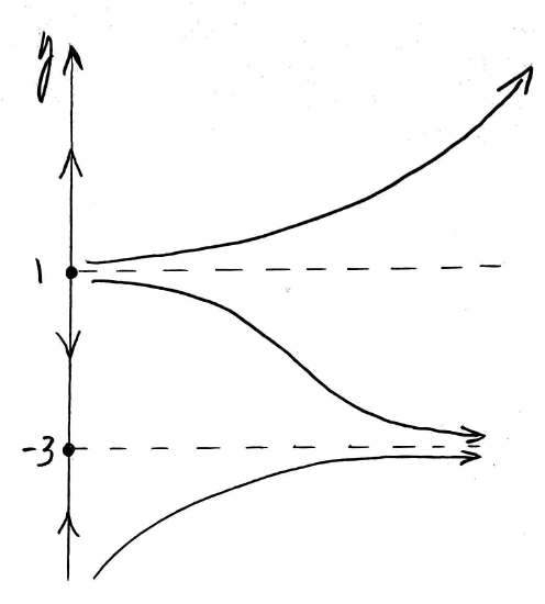
First we need to create a sequence of phase portraits for various values of the parameter \(a.\) In Example \(\PageIndex{1}\) above, we created three of these phase portraits. We can use a similar approach to find the phase portrait for \(a = -3,\) noting that \(\dfrac{dy}{dt}=y^2 + 2y - 3\) factors nicely.
Here we have
\[\begin{align*} y^2 + 2y - 3 &= 0 \\[4pt]
(y+3)(y-1) &= 0 \end{align*}\]
So \(y = -3\) and \(y = 1\) are critical numbers of this ODE and correspond to two equilibrium solutions of the ODE. Testing values of \(y\) in the corresponding intervals of the \(y\)-axis gives us the following phase portrait. (Remember that the phase portrait includes the phase line on the left and representative curves along with the equilibrium solutions on the right.)
Now we can put the four phase lines we've created together on a plane where the horizontal axis represents the parameter \(a\) and the vertical axis is the dependent variable \(y\) (this one is the same as the phase lines above). We can fill in a few additional phase lines using the interactive figure in Figure \(\PageIndex{4}\) above. Note that in addition to using dashed lines for the individual phase lines, we also indicated critical points with stable equilibria with solid points and critical points with unstable equilibria with open points. From Figure \(\PageIndex{2}\) above, you can see that the single critical point at \(y = -1\) when \(a = 1\) is semi-stable. We'll indicate this by making it half-open on the side where the curve is diverging from this equilibrium solution and half-solid on the side where the curve is converging to the equilibrium solution (so we get a half-solid point there).
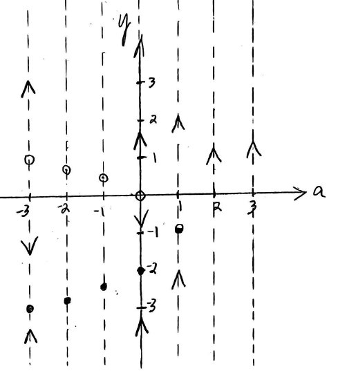
To finish the bifurcation diagram we'll connect solid critical points with a solid curve and use a dashed curve to connect the open critical points.
This bifurcation diagram gives us a visual representation of all the possible phase lines for \(-4 \le a \le 3.\)
As a way to visually explore this bifurcation diagram (and to see how it is different from the interactive graph of \(\dfrac{dy}{dt} = f(y)\) shown in Figure \(\PageIndex{4},\) use the slider to vary the value of \(a\) in interactive Figure \(\PageIndex{10}\) below. Note that it contains this bifurcation diagram and also the corresponding phase portrait, including representative solution curves. Observe how the representative solution curves change as you vary the value of the parameter \(a.\)
Now that you've seen one full example of the process, let's summarize the steps you can use to create a bifurcation diagram for any given differential equation with a single parameter.
To create a bifurcation diagram for a given differential equation containing a single parameter \(a\):
- You may find it helpful to do the following as you begin:
- Explore the graph of \(\dfrac{dy}{dt} = f(y)\) to locate any potential bifurcations graphically.
- Create a phase portrait for at least one convenient value of the parameter \(a\) (or whatever parameter is used).
- You will typically be required to show the algebraic approach to locate/prove any bifurcation points.
- Next you will likely be asked to show a sequence of phase lines (or full phase portraits) to illustrate the behavior of the ODE for values of the parameter that lie at or on either side of any bifurcation points you determined in Step 2. It is very helpful even at this step to include open circles at critical points where the ODE has unstable equilibrium solutions, solid points at critical points where the ODE has stable equilibrium solutions and half-solid/half-open circles at points for which the ODE has semi-stable equilibrium solutions (placing the solid part on the stable side).
- Draw a pair of coordinate axes where the vertical axis is labeled with the dependent variable (often \(y\)) and the horizontal axis is labeled with the parameter name (.e.g., \(a\)). Add the phase lines from Step 3 (and possibly add some new ones) at each "nice" (and/or relevant) value of the parameter (on the horizontal axis) as shown in Figure \(\PageIndex{9}\) above.
- Finally, connect the stable (solid) critical points with a solid curve and connect unstable (open) critical points with a dashed curve.
Now, note that in Example \(\PageIndex{4}\) both the bifurcation diagram in Figure \(\PageIndex{9}\) and the corresponding graph of \(\dfrac{dy}{dt} = f(y)\) shown in Figure \(\PageIndex{4}\) are horizontal parabolas. This does not mean that the bifurcation diagram of an ODE with a single parameter will always have the same shape as the graph of \(\dfrac{dy}{dt} = f(y).\) You will see how different these graphs can look when you create the bifurcation diagram in Exercise \(\PageIndex{2}\) below.
Use the steps listed above to draw the bifurcation diagram for the differential equation below with parameter \(a.\)
\[\dfrac{dy}{dt}=y^3 + ay^2 + y \nonumber\]
- Answer
-
Following the steps from the summary of this process given above:
1. We have already explored this differential equation graphically above in Exercise \(\PageIndex{1}.\) If you have not yet tried this exercise, you may want to start there. If you were doing this problem on your own, you may want to try to create a phase portrait for one of the values that you found interesting from exploring the ODE graphically.
2. Next we'll examine the differential equation algebraically to look for bifurcation points. As mentioned above, this work is generally always required to be shown to earn full credit on problem asking for a bifurcation diagram.
Determining bifurcation points:
First we set \(f(y) = 0\) and solve for \(y\):
\[\begin{align*} y^3 + ay^2 + y &= 0 \\[4pt]
y(y^2+ay +1) &= 0 \end{align*}\]This means that either \(y = 0\) or \(y^2+ay +1 = 0.\) Solving this second equation using the quadratic formula, we obtain
\[\begin{align*} y &= \dfrac{-a \pm \sqrt{a^2 - 4(1)(1)}}{2} \\[5pt]
&= \dfrac{-a \pm \sqrt{a^2 - 4}}{2} \end{align*}\]Remembering that \(y = 0\) is always an equilibrium solution here, and this quadratic equation has 0, 1, or 2 solutions depending on the value of the discriminant \(a^2 - 4,\) we can see that the total number of equilibrium solutions of the ODE will be 1, 2, or 3, depending on the value of the expression \(a^2 - 4\) under the radical.
Case 1: If \(a^2 - 4 = 0 \quad \rightarrow \quad a = -2 \text{ or } a = 2,\) there are two equilibrium solutions: \( y = 0\) and \(y = -\frac{a}{2}.\)
Case 2: If \(a^2 - 4 > 0 \quad \rightarrow \quad a < -2 \text{ or } a > 2,\) there are three equilibrium solutions: \( y = 0\) and \(\dfrac{-a \pm \sqrt{a^2 - 4}}{2}.\)
Case 3: If \(a^2 - 4 < 0 \quad \rightarrow \quad -2 < a < 2,\) there is only the one equilibrium solution \(y = 0\), since \(y\) would be complex imaginary in the quadratic equation above resulting in no additional (real-valued) equilibrium solutions.
We see that \(a = -2\) and \(a = 2\) are both transition points where the number of equilibrium solutions changes from \(1\) to \(2\) to \(3,\) as we adjust the value of \(a\) from numbers between \(-2\) and \(2\) to \(a = -2\) or \(a = 2\) to numbers that are more than \(2\) units from \(0\) on the number line, i.e., to values of \(a\) in \((\infty, -2)\) or \((2, \infty).\)
This means that \(a = -2\) and \(a = 2\) are the bifurcation points of this ODE!
3. Now we need a collection of phase lines to help us draw the bifurcation diagram. Ideally, we will want one for every "nice" value of the parameter on a range that includes all the bifurcation points and a reasonable distance past them on either side (to the left and right). For this example, let's take the integer values of \(a\) from \(-4\) to \(4\). From our work above, we know that all values between -2 and 2 will have the same phase line though, so we really only need to consider one value of \(a\) in this interval at this step. We'll choose \(a = 0\) as an easy value to use here.
Phase line 1: \(a = 0\)
Here \[\dfrac{dy}{dt}=y^3 + y \nonumber\]
Solving for the equilibrium solution(s), we set the ODE equal to \(0,\) factor, and solve for \(y.\)
\[\begin{align*} y^3 + y &= 0 \\[5pt]
y(y^2 + 1) &= 0 \\[5pt]
\text{so } y = 0 & \text{ or }y^2 + 1 = 0\end{align*}\]Since \(y = 0\) is the only real solution here, \(y = 0\) is our only critical point (equilibrium solution).
Next we check the sign of \(\dfrac{dy}{dt}\) for a value of \(y\) below \(0\) and for a value greater than \(0.\)
\[\begin{align*} \text{At }y = -1, \quad \dfrac{dy}{dt} \Bigg|_{y \,=\, -1} &= (-1)^3 + (-1) = -2 < 0. & & \text{So solutions will be decreasing for }y<0.\\[5pt]
\text{At }y = 1, \quad \dfrac{dy}{dt} \Bigg|_{y\,=\, 1} &= (1)^3 + 1 = 2 > 0. & & \text{So solutions will also be increasing for }y>0.\end{align*} \]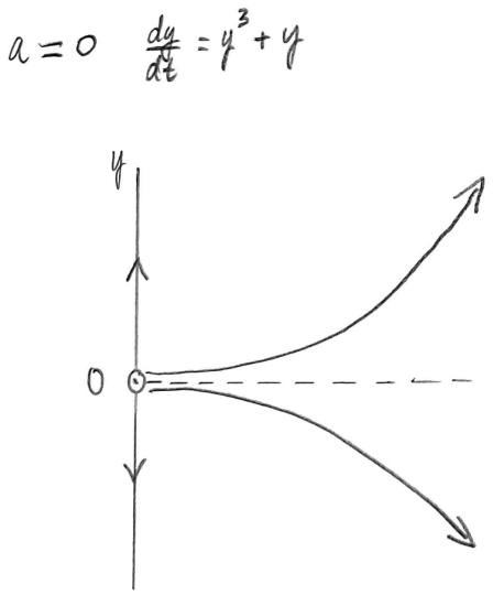
Figure \(\PageIndex{10}\): Phase line and representative solution curves for \(\dfrac{dy}{dt}=y^3 + y\), i.e., for \(a = 0\) Phase line 2: \(a = 2\)
Here \[\dfrac{dy}{dt}= y^3 + 2y^2 + y \nonumber\]
Solving for the equilibrium solution(s), we set the ODE equal to \(0,\) factor, and solve for \(y.\)
\[\begin{align*} y^3 + 2y^2 + y &= 0 \\[5pt]
y(y^2 + 2y + 1) &= 0 \\[5pt]
y(y + 1)^2 &= 0 \\[5pt]
\text{so } y = 0 & \text{ or }y = -1\end{align*}\]Thus \(y = 0\) and \(y = -1\) are our critical points that give us equilibrium solutions.
Next we check the sign of \(\dfrac{dy}{dt}\) for a value of \(y\) below \(-1\), between \(-1\) and \(0\) and for a value greater than \(0.\) We'll use the factored form, since it's easier to work with here.
\[\begin{align*} \text{At }y = -2, \quad \dfrac{dy}{dt} \Bigg|_{y \,=\, -2} &= -2(-2+1)^2 = -2 < 0. & & \text{So solutions will be decreasing for }y<-1.\\[5pt]
\text{At }y = -0.5, \quad \dfrac{dy}{dt} \Bigg|_{y \,=\, -0.5} &= -0.5(-0.5+1)^2 = -\tfrac{1}{8} < 0. & & \text{So solutions will be decreasing for }-1<y<0.\\[5pt]
\text{At }y = 1, \quad \dfrac{dy}{dt} \Bigg|_{y\,=\, 1} &= 1(1+1)^2 = 4 > 0. & & \text{So solutions will also be increasing for }y>0.\end{align*} \]See the left phase portrait in Figure \(\PageIndex{11}\) below.
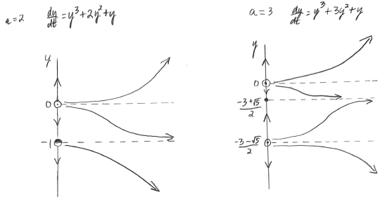
Figure \(\PageIndex{11}\): Phase lines and representative solution curves for \(\dfrac{dy}{dt}=y^3 + ay^2 + y,\) for \(a = 2\) and \(a = 3.\) Phase line 3: \(a = 3\)
Here \[\dfrac{dy}{dt}= y^3 + 3y^2 + y \nonumber\]
Solving for the equilibrium solution(s), we set the ODE equal to \(0,\) factor, and solve for \(y.\) Note that when we factor, we are left with a non-factorable trinomial factor. We use the quadratic formula to find its two real zeros.
\[\begin{align*} y^3 + 3y^2 + y &= 0 \\[5pt]
y(y^2 + 3y + 1) &= 0 \\[5pt]
\text{so } y = 0 & \text{ or }y^2 + 3y + 1 = 0\end{align*}\]Using the quadratic formula to solve the trinomial equation on the right,
\[\begin{align*} y &= \dfrac{-3 \pm \sqrt{9 - 4(1)(1)}}{2} \\[5pt]
&= \dfrac{-3 \pm \sqrt{5}}{2} \end{align*}\]So we end up with three critical points here that each give us equilibrium solutions. These are \(y = 0,\) \(y = \dfrac{-3 -\sqrt{5}}{2} \approx -2.62,\) and \(y = \dfrac{-3 +\sqrt{5}}{2} \approx -0.38.\)
Next we check the sign of \(\dfrac{dy}{dt}\) for a value of \(y\) below \( \dfrac{-3 -\sqrt{5}}{2} \), between \(\dfrac{-3 -\sqrt{5}}{2}\) and \(\dfrac{-3 +\sqrt{5}}{2}\), between \(\dfrac{-3 +\sqrt{5}}{2}\) and \(0\), and for a value greater than \(0.\)
\[\begin{align*} \text{At }y = -3, \quad \dfrac{dy}{dt} \Bigg|_{y \,=\, -3} &= (-3)^3 + 3(-3)^2 + (-3) = -3 < 0. & & \text{So solutions will be decreasing for }y< \dfrac{-3 -\sqrt{5}}{2} .\\[5pt]
\text{At }y = -1, \quad \dfrac{dy}{dt} \Bigg|_{y \,=\, -1} &= (-1)^3 + 3(-1)^2 + (-1) = 1 > 0. & & \text{So solutions will be increasing for }\dfrac{-3 -\sqrt{5}}{2}<y<\dfrac{-3 +\sqrt{5}}{2}.\\[5pt]
\text{At }y = -0.1, \quad \dfrac{dy}{dt} \Bigg|_{y \,=\, -0.1} &= (-0.1)^3 + 3(-0.1)^2 + (-0.1) \\[5pt]
&= -0.001 + 0.03 - 0.1 = -0.71 < 0. & & \text{So solutions will be decreasing for }\dfrac{-3 +\sqrt{5}}{2}<y<0.\\[5pt]
\text{At }y = 1, \quad \dfrac{dy}{dt} \Bigg|_{y\,=\, 1} &= (1)^3 + 3(1)^2 + 1 = 4 > 0. & & \text{So solutions will also be increasing for }y>0.\end{align*} \]See the right phase portrait in Figure \(\PageIndex{11}\) above.
Similar work will produce the additional phase portraits shown in Figures \(\PageIndex{12}\) and \(\PageIndex{13}\). Note that some symmetry (about the origin) shows up in our results.
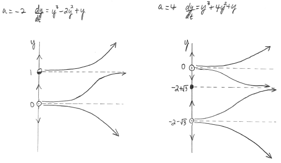
Figure \(\PageIndex{12}\): Phase lines and representative solution curves for \(\dfrac{dy}{dt}=y^3 + ay^2 + y,\) for \(a = -2\) and \(a = 4.\) 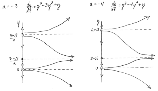
Figure \(\PageIndex{13}\): Phase lines and representative solution curves for \(\dfrac{dy}{dt}=y^3 + ay^2 + y,\) for \(a = -3\) and \(a = -4.\) 4. & 5. Figure \(\PageIndex{14}\) shows the completed bifurcation diagram for this ODE. Note that there are three parts to the plot of the bifurcation diagram, including a dashed line along the \(x\)-axis representing the equilibrium solution \(y = 0.\)
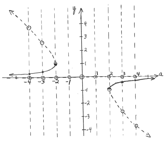
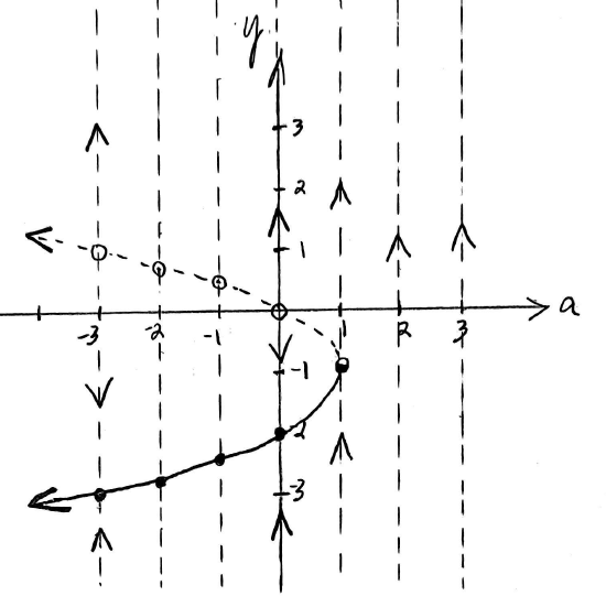
Figure \(\PageIndex{14}\): Completed bifurcation diagram for \(\dfrac{dy}{dt}=y^3 + ay^2 + y.\)
Bifurcations like these can occur in many real-life situations, so it is important to be aware of them. It's also vital to be able to identify them and to be able to create bifurcation diagrams to see more clearly how they affect the solutions of the differential equation that model the situation.