
Constrained Optimization
- Page ID
- 21133
\( \newcommand{\vecs}[1]{\overset { \scriptstyle \rightharpoonup} {\mathbf{#1}} } \)
\( \newcommand{\vecd}[1]{\overset{-\!-\!\rightharpoonup}{\vphantom{a}\smash {#1}}} \)
\( \newcommand{\dsum}{\displaystyle\sum\limits} \)
\( \newcommand{\dint}{\displaystyle\int\limits} \)
\( \newcommand{\dlim}{\displaystyle\lim\limits} \)
\( \newcommand{\id}{\mathrm{id}}\) \( \newcommand{\Span}{\mathrm{span}}\)
( \newcommand{\kernel}{\mathrm{null}\,}\) \( \newcommand{\range}{\mathrm{range}\,}\)
\( \newcommand{\RealPart}{\mathrm{Re}}\) \( \newcommand{\ImaginaryPart}{\mathrm{Im}}\)
\( \newcommand{\Argument}{\mathrm{Arg}}\) \( \newcommand{\norm}[1]{\| #1 \|}\)
\( \newcommand{\inner}[2]{\langle #1, #2 \rangle}\)
\( \newcommand{\Span}{\mathrm{span}}\)
\( \newcommand{\id}{\mathrm{id}}\)
\( \newcommand{\Span}{\mathrm{span}}\)
\( \newcommand{\kernel}{\mathrm{null}\,}\)
\( \newcommand{\range}{\mathrm{range}\,}\)
\( \newcommand{\RealPart}{\mathrm{Re}}\)
\( \newcommand{\ImaginaryPart}{\mathrm{Im}}\)
\( \newcommand{\Argument}{\mathrm{Arg}}\)
\( \newcommand{\norm}[1]{\| #1 \|}\)
\( \newcommand{\inner}[2]{\langle #1, #2 \rangle}\)
\( \newcommand{\Span}{\mathrm{span}}\) \( \newcommand{\AA}{\unicode[.8,0]{x212B}}\)
\( \newcommand{\vectorA}[1]{\vec{#1}} % arrow\)
\( \newcommand{\vectorAt}[1]{\vec{\text{#1}}} % arrow\)
\( \newcommand{\vectorB}[1]{\overset { \scriptstyle \rightharpoonup} {\mathbf{#1}} } \)
\( \newcommand{\vectorC}[1]{\textbf{#1}} \)
\( \newcommand{\vectorD}[1]{\overrightarrow{#1}} \)
\( \newcommand{\vectorDt}[1]{\overrightarrow{\text{#1}}} \)
\( \newcommand{\vectE}[1]{\overset{-\!-\!\rightharpoonup}{\vphantom{a}\smash{\mathbf {#1}}}} \)
\( \newcommand{\vecs}[1]{\overset { \scriptstyle \rightharpoonup} {\mathbf{#1}} } \)
\(\newcommand{\longvect}{\overrightarrow}\)
\( \newcommand{\vecd}[1]{\overset{-\!-\!\rightharpoonup}{\vphantom{a}\smash {#1}}} \)
\(\newcommand{\avec}{\mathbf a}\) \(\newcommand{\bvec}{\mathbf b}\) \(\newcommand{\cvec}{\mathbf c}\) \(\newcommand{\dvec}{\mathbf d}\) \(\newcommand{\dtil}{\widetilde{\mathbf d}}\) \(\newcommand{\evec}{\mathbf e}\) \(\newcommand{\fvec}{\mathbf f}\) \(\newcommand{\nvec}{\mathbf n}\) \(\newcommand{\pvec}{\mathbf p}\) \(\newcommand{\qvec}{\mathbf q}\) \(\newcommand{\svec}{\mathbf s}\) \(\newcommand{\tvec}{\mathbf t}\) \(\newcommand{\uvec}{\mathbf u}\) \(\newcommand{\vvec}{\mathbf v}\) \(\newcommand{\wvec}{\mathbf w}\) \(\newcommand{\xvec}{\mathbf x}\) \(\newcommand{\yvec}{\mathbf y}\) \(\newcommand{\zvec}{\mathbf z}\) \(\newcommand{\rvec}{\mathbf r}\) \(\newcommand{\mvec}{\mathbf m}\) \(\newcommand{\zerovec}{\mathbf 0}\) \(\newcommand{\onevec}{\mathbf 1}\) \(\newcommand{\real}{\mathbb R}\) \(\newcommand{\twovec}[2]{\left[\begin{array}{r}#1 \\ #2 \end{array}\right]}\) \(\newcommand{\ctwovec}[2]{\left[\begin{array}{c}#1 \\ #2 \end{array}\right]}\) \(\newcommand{\threevec}[3]{\left[\begin{array}{r}#1 \\ #2 \\ #3 \end{array}\right]}\) \(\newcommand{\cthreevec}[3]{\left[\begin{array}{c}#1 \\ #2 \\ #3 \end{array}\right]}\) \(\newcommand{\fourvec}[4]{\left[\begin{array}{r}#1 \\ #2 \\ #3 \\ #4 \end{array}\right]}\) \(\newcommand{\cfourvec}[4]{\left[\begin{array}{c}#1 \\ #2 \\ #3 \\ #4 \end{array}\right]}\) \(\newcommand{\fivevec}[5]{\left[\begin{array}{r}#1 \\ #2 \\ #3 \\ #4 \\ #5 \\ \end{array}\right]}\) \(\newcommand{\cfivevec}[5]{\left[\begin{array}{c}#1 \\ #2 \\ #3 \\ #4 \\ #5 \\ \end{array}\right]}\) \(\newcommand{\mattwo}[4]{\left[\begin{array}{rr}#1 \amp #2 \\ #3 \amp #4 \\ \end{array}\right]}\) \(\newcommand{\laspan}[1]{\text{Span}\{#1\}}\) \(\newcommand{\bcal}{\cal B}\) \(\newcommand{\ccal}{\cal C}\) \(\newcommand{\scal}{\cal S}\) \(\newcommand{\wcal}{\cal W}\) \(\newcommand{\ecal}{\cal E}\) \(\newcommand{\coords}[2]{\left\{#1\right\}_{#2}}\) \(\newcommand{\gray}[1]{\color{gray}{#1}}\) \(\newcommand{\lgray}[1]{\color{lightgray}{#1}}\) \(\newcommand{\rank}{\operatorname{rank}}\) \(\newcommand{\row}{\text{Row}}\) \(\newcommand{\col}{\text{Col}}\) \(\renewcommand{\row}{\text{Row}}\) \(\newcommand{\nul}{\text{Nul}}\) \(\newcommand{\var}{\text{Var}}\) \(\newcommand{\corr}{\text{corr}}\) \(\newcommand{\len}[1]{\left|#1\right|}\) \(\newcommand{\bbar}{\overline{\bvec}}\) \(\newcommand{\bhat}{\widehat{\bvec}}\) \(\newcommand{\bperp}{\bvec^\perp}\) \(\newcommand{\xhat}{\widehat{\xvec}}\) \(\newcommand{\vhat}{\widehat{\vvec}}\) \(\newcommand{\uhat}{\widehat{\uvec}}\) \(\newcommand{\what}{\widehat{\wvec}}\) \(\newcommand{\Sighat}{\widehat{\Sigma}}\) \(\newcommand{\lt}{<}\) \(\newcommand{\gt}{>}\) \(\newcommand{\amp}{&}\) \(\definecolor{fillinmathshade}{gray}{0.9}\)In this section, we will consider some applications of optimization. Applications of optimization almost always involve some kind of constraints or boundaries.
Anytime we have a closed region or have constraints in an optimization problem the process we'll use to solve it is called constrained optimization. In this section we will explore how to use what we've already learned to solve constrained optimization problems in two ways. In the next section we will learn a different approach called the Lagrange multiplier method that can be used to solve many of the same (and some additional) constrained optimization problems.
We will first look at a way to rewrite a constrained optimization problem in terms of a function of two variables, allowing us to find its critical points and determine optimal values of the function using the second partials test. We will then consider another approach to determining absolute extrema of a function of two variables on a closed region, where we can write each boundary as a function of \(x\).
Applications of Optimization - Approach 1: Using the Second Partials Test
Example \(\PageIndex{1}\): A Box Problem
A closed cardboard box is constructed from different materials. If the material for the base of the box costs $2 per square foot, and the side/top material costs $1 per square foot, find the dimensions of the largest box that can be created for $36.
Solution
Consider the box shown in the diagram.
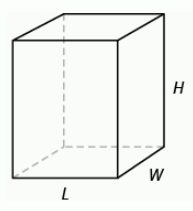
Our first task will be to come up with the objective function (what we are trying to optimize). Here this is the volume of the box (see that we were asked for the "largest box"). Using the variables from the diagram, we have:
\[\text{Objective Function}:\qquad V=LWH\]
Now we need to write the constraint using the same variables. The constraint here is the cost of the materials for the box. Since the cost of the material in the bottom of the box is twice the cost of the materials in the rest of the box, we'll need to account for this in the constraint. We have that the cost of the sides is $1 per square foot, and so the cost of the bottom of the box must be $2 per square foot. Now we need to write an expression for the area of the bottom of the box and another for the area of the sides and top of the box.
\[\text{Area of bottom of box}=LW\qquad\text{Area of sides of box and the top}=2LH + 2WH + LW\]
Now we can put the costs of the respective material together with these areas to write the cost constraint:
\[\text{Cost Constraint}: \qquad 2LW + (2LH + 2WH + LW) = 36 \quad\rightarrow\quad 3LW + 2LH + 2WH = 36\]
Note that there are also some additional implied constraints in this problem. That is, we know that \(L \ge 0, W \ge 0\), and \(H\ge 0\).
This constraint can be used to reduce the number of variables in the objective function, \(V=LWH\), from three to two. We can choose to solve the constraint for any convenient variable, so let's solve it for \(H\). Then,
\[\begin{align*} 3LW + 2LH + 2WH &= 36 \\[5pt]
\rightarrow \quad 2H(L+W)&=36 - 3LW \\[5pt]
\rightarrow \quad H &= \frac{36 - 3LW}{2(L+W)}\end{align*}\]
Substituting this result into the objective function (replacing \(H\)), we obtain:
\[V(L,W) = LW\left( \frac{36 - 3LW}{2(L+W)}\right)= \frac{36LW - 3L^2W^2}{2(L+W)}\]
Now that we have the volume expressed as a function of just two variables, we can find its critical points (feasible for this situation) and then use the second partials test to confirm that we obtain a relative maximum volume at one of these points.
Finding Critical Points:
First we find the partial derivatives of \(V\): \[\begin{align*} V_{L}(L,W) &= \frac{2(L+W)(36W-6LW^2) - 2(36LW-3L^2W^2)}{4(L+W)^2} & & \text{by the Quotient Rule} \\[5pt]
&= \frac{(L+W)(36W-6LW^2) - (36LW-3L^2W^2)}{2(L+W)^2} & & \text{Canceling a common factor of 2} \\[5pt]
&= \frac{36LW-6L^2W^2+36W^2-6LW^3 - 36LW+3L^2W^2}{2(L+W)^2} & & \text{Simplifying the numerator} \\[5pt]
&= \frac{36W^2-6LW^3 -3L^2W^2}{2(L+W)^2} & & \text{Collecting like terms} \\[5pt]
&= \frac{W^2(36 - 6LW -3L^2)}{2(L+W)^2} & & \text{Factoring out}\,W^2\end{align*}\]
Similarly, we find that
\[V_{W}(L,W) = \frac{L^2(36 - 6LW -3W^2)}{2(L+W)^2}\]
Setting these partial derivatives both equal to zero, we note that the denominators cannot make either partial equal zero. We can then write the nonlinear system:
\[\begin{align*} W^2(36 - 6LW -3L^2) &=0 \\[5pt]
L^2(36 - 6LW -3W^2) &= 0\end{align*}\]
Note that if not for the fact that in this application we know that the variables \(L\) and \(W\) are non-negative, we would find that this function has critical points anywhere the denominator of these partials is equal to \(0\), i.e., when \(L = -W\). That is, all points on the line \(L = -W\) would be critical points of this function. But since this is not possible here, we can ignore it and go on.
To solve the system above, we first note that both equations are factored and set equal to zero. Using the zero-product property, we know the first equation tells us that either
\[W=0\quad\text{or}\quad 36 - 6LW -3L^2=0\]
The second equation tells us that
\[L=0\quad\text{or}\quad 36 - 6LW -3W^2=0\]
Taking the various combinations here, we find
\(W=0\) and \(L=0\quad\rightarrow\quad\)Critical point: (0, 0). However, we see that this point also makes the denominator of the partials zero, making it a critical point of the second kind. We also see that with these dimensions the other constraint could not be true. We'd end up with a cost of $0, not $36.
\(W=0\) and \(36 - 6LW -3W^2=0\) is impossible, since when we put zero in for \(W\) in the second equation, we obtain the contradiction, \(36 = 0\).
\(36 - 6LW -3L^2=0\) and \(L=0\) is also impossible, since when we put zero in for \(L\) in the first equation, we again obtain the contradiction, \(36 = 0\).
Finally, considering the combination of the last two equations we have the system:
\[\begin{align*} 36 - 6LW -3W^2&=0\\[5pt] 36 - 6LW -3L^2&=0\end{align*}\]
Multiplying through the bottom equation by \(-1\), we have
\[\begin{align*} 36 - 6LW -3W^2&=0\\[5pt] -36 + 6LW +3L^2&=0\end{align*}\]
Adding the two equations eliminates the first two terms on the left side of each equation, yielding
\[3L^2 - 3W^2=0 \quad\rightarrow\quad 3(L - W)(L+W) = 0\]
So we have that
\[L=W \quad\text{or}\quad L=-W\]
Since we know that none of the dimensions can be negative we can reject \(L=-W\). This leaves us with the result that \(L=W\).
Substituting this into the first equation of our system above (we could have used either one), gives us
\[\begin{align*} 36 - 6W^2 - 3W^2 &= 0 \\[5pt]
36 - 9W^2 &= 0 \\[5pt]
9(4 - W^2) &=0 \\[5pt]
9(2-W)(2+W) &=0 \end{align*}\]
From this equation we see that either \(W=2\) or \(W=-2\). Since the width cannot be negative, we reject \(W=-2\) and conclude that \(W=2\) ft.
Then, since \(L=W\), we know that \(L=2\) ft also.
Using the formula we found for \(H\) above, we find that the corresponding height is
\[H = \frac{36 - 3(2)(2)}{2(2+2)} = \frac{24}{8} =3 \,\text{ft}\]
This gives a volume of \(V = 2 \cdot 2 \cdot 3 = 12 \,\text{ft}^3\).
Note that the critical point we just found was actually \((2, 2)\). This is the only feasible critical point of the function \(V\).
Now we just have to use the second partials test to prove that we obtain a relative maximum here.
Second Partials Test:
First we need to determine the second partials of \(V(L,W)\), i.e., \(V_{LL}, V_{WW},\) and \(V_{LW}\).
\[\begin{align*} V_{LL}(L,W) &= \frac{2(L+W)^2(-6W^3-6LW^2)-4(L+W)(36W^2-6LW^3-3L^2W^2)}{4(L+W)^4} \\[5pt]
&= \frac{4(L+W)\Big[(L+W)(-3W^3-3LW^2)-36W^2+6LW^3+3L^2W^2\Big]}{4(L+W)^4} \\[5pt]
&= \frac{-3LW^3-3L^2W^2-3W^4-3LW^3-36W^2+6LW^3+3L^2W^2}{(L+W)^3} \\[5pt]
&= \frac{-3W^4-36W^2}{(L+W)^3} \end{align*}\]
Similarly, we find
\[V_{WW}(L,W) =\frac{-3L^4-36L^2}{(L+W)^3}\]
And the mixed partial
\[\begin{align*} V_{LW}(L,W) &= \frac{2(L+W)^2(72W-18LW^2-6L^2W)-4(L+W)(36W^2-6LW^3-3L^2W^2)}{4(L+W)^4} \\[5pt]
&= \frac{4(L+W)\Big[(L+W)(36W-9LW^2-3L^2W)-36W^2+6LW^3+3L^2W^2\Big]}{4(L+W)^4} \\[5pt]
&= \frac{36LW+36W^2-9L^2W^2-9LW^3-3L^3W - 3L^2W^2 - 36W^2 + 6LW^3 + 3L^2W^2}{(L+W)^3} \\[5pt]
&= \frac{36LW - 3LW^3 - 9L^2W^2 - 3L^3W}{(L+W)^3} \end{align*}\]
Now we can calculate the discriminant at the critical point:
\[\begin{align*} D(2,2) &= V_{LL}(2,2)\cdot V_{WW}(2,2) - \big[V_{LW}(2,2)\big]^2 \\[5pt]
&= (-3)(-3) - \left(-\frac{3}{2}\right)^2 = 9 - \frac{9}{4} = \frac{27}{4} > 0 \end{align*}\]
Since \(D>0\) and \(V_{LL}(2,2) = -3 < 0\), we know that \(V(L, W)\) is concave down at this critical point and thus has a relative maximum of \(12\) there.
Therefore, we know that the box of maximum volume that costs \($36\) to make will have a volume of \(V = 2\,\text{ft} \cdot 2\,\text{ft} \cdot 3\,\text{ft} = 12 \,\text{ft}^3\).
Finding Absolute Extrema on a Closed, Bounded Region
When optimizing functions of one variable such as \(y=f(x)\), we used the Extreme Value Theorem. It said that over a closed interval \(I\), a continuous function has both an absolute maximum value and an absolute minimum value. To find these maximum and minimum values, we evaluated \(f\) at all critical points in the interval, as well as at the endpoints (the "boundaries'') of the interval.
A similar theorem and procedure applies to functions of two variables. When working with a function of two variables, the closed interval is replaced by a closed, bounded region. A region is bounded if all the points in that region can be contained within a disk (or ball) of finite radius. Just as a continuous function of one variable was guaranteed to have an absolute maximum and an absolute minimum on a closed interval, a continuous function of two variables will attain an absolute maximum and absolute minimum value over a closed region (see the following theorem).
We can find these values by evaluating the function at its critical points in the region and at the critical values and endpoints of traces formed on the boundaries of the region. First, we need to find the critical points of the function that lie inside the region and calculate the corresponding function values. Then, it is necessary to find the maximum and minimum values of the function on the boundaries of the region. When we have all these values, the largest function value corresponds to the absolute (global) maximum and the smallest function value corresponds to the absolute (global) minimum.
First, however, we need to be assured that such values exist. The following theorem does this.
Theorem \(\PageIndex{1}\): Extreme Value Theorem
Let \(z=f(x,y)\) be a continuous function on a closed, bounded region \(S\). Then \(f\) has an absolute maximum value at some point in \(S\) and an absolute minimum value at some point in \(S\).
The proof of this theorem is a direct consequence of the extreme value theorem and Fermat’s theorem. In particular, if either extremum is not located on the boundary of \(S\), then it is located at an interior point of \(S\). But an interior point \((x_0,y_0)\) of \(S\) that’s an absolute extremum is also a local extremum; hence, \((x_0,y_0)\) is a critical point of \(f\) by Fermat’s theorem. Therefore the only possible values for the global extrema of \(f\) on \(S\) are the extreme values of \(f\) on the interior or boundary of \(S\).
Now that we know any continuous function \(f\) defined on a closed, bounded region will have global extreme values on that region, let's summarize how to find them.
Finding Extreme Values of a Function of Two Variables
Assume \(z=f(x,y)\) is a differentiable function of two variables defined on a closed, bounded region \(S\). Then \(f\) will attain the absolute maximum value and the absolute minimum value, which are, respectively, the largest and smallest values found among the following:
- The values of \(f\) at the critical points of \(f\) in \(S\).
- The values of \(f\) on the boundary of \(S\).
Now let's see how this works in an example.
Example \(\PageIndex{2}\): Finding Extrema on a Closed, Bounded Region
Let \(f(x,y) = x^2-y^2+5\) and let the region \(S\) be the triangle with vertices \((-1,-2)\), \((0,1)\) and \((2,-2)\), including its interior. Find the absolute maximum and absolute minimum values of \(f\) on \(S\).
SOLUTION
It can help to see a graph of \(f\) along with the region \(S\). In Figure \(\PageIndex{1}\)(a) the triangle defining \(S\) is shown in the \(xy\)-plane (using dashed red lines). Above it is the surface of \(f\). Here we are only concerned with the portion of \(f\) enclosed by the "triangle'' on its surface. Note that the triangular region forming our constrained region \(S\) in the \(xy\)-plane has been projected up onto the surface above it.
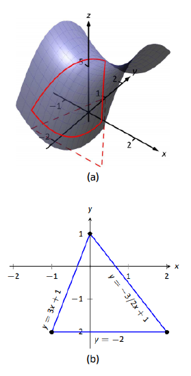
Figure \(\PageIndex{1}\): Plotting the surface of \(f\) along with the restricted domain \(S\).
We begin by finding the critical points of \(f\). With \(f_x(x,y) = 2x\) and \(f_y(x,y) = -2y\), we find only one critical point, at \((0,0)\).
We now find the maximum and minimum values that \(f\) attains along the boundary of \(S\), that is, along the edges of the triangle. In Figure \(\PageIndex{1}\)(b) we see the triangle sketched in the plane with the equations of the lines forming its edges labeled.
Start with the bottom edge, along the line \(y=-2\). If \(y\) is \(-2\), then on the surface, we are considering points \(f(x,-2)\); that is, our function reduces to \(f(x,-2) = x^2-(-2)^2+5 = x^2+1=f_1(x)\). We want to maximize/minimize \(f_1(x)=x^2+1\) on the interval \([-1,2]\). To do so, we evaluate \(f_1(x)\) at its critical points and at the endpoints.
The critical points of \(f_1\) are found by setting its derivative equal to 0:
\[f'_1(x)=0\qquad \Rightarrow x=0.\]
Evaluating \(f_1\) at this critical point, and at the endpoints of \([-1,2]\) gives:
\[\begin{align*}
f_1(-1) = 2 \qquad&\Rightarrow & f(-1,-2) &= 2\\
f_1(0) = 1 \qquad&\Rightarrow & f(0,-2) &= 1\\
f_1(2) = 5 \qquad&\Rightarrow & f(2,-2) &= 5.
\end{align*}\]
Notice how evaluating \(f_1\) at a point is the same as evaluating \(f\) at its corresponding point.
We need to do this process twice more, for the other two edges of the triangle.
Along the left edge, along the line \(y=3x+1\), we substitute \(3x+1\) in for \(y\) in \(f(x,y)\):
\[f(x,y) = f(x,3x+1) = x^2-(3x+1)^2+5 = -8x^2-6x+4 = f_2(x).\]
We want the maximum and minimum values of \(f_2\) on the interval \([-1,0]\), so we evaluate \(f_2\) at its critical points and the endpoints of the interval. We find the critical points:
\[f'_2(x) = -16x-6=0 \qquad \Rightarrow \qquad x=-\tfrac{3}{8}.\]
Evaluate \(f_2\) at its critical point and the endpoints of \([-1,0]\):
\[\begin{align*}
f_2(-1) &= 2 & &\Rightarrow & f(-1,-2) &= 2\\
f_2\left(-\tfrac{3}{8}\right) &= \tfrac{41}{8}=5.125 & &\Rightarrow & f\left(-\tfrac{3}{8},-0.125\right) &= 5.125\\
f_2(0) &= 1 & &\Rightarrow & f(0,1) &= 4.
\end{align*}\]
Finally, we evaluate \(f\) along the right edge of the triangle, where \(y = -\frac{3}{2}x+1\).
\[f(x,y) = f\left(x,-\tfrac{3}{2}x+1\right) = x^2-\left(-\tfrac{3}{2}x+1\right)^2+5 = -\tfrac{5}{4}x^2+3x+4=f_3(x).\]
The critical points of \(f_3(x)\) are:
\[f'_3(x) = 0 \qquad \Rightarrow \qquad x=\tfrac{6}{5}=1.2.\]
We evaluate \(f_3\) at this critical point and at the endpoints of the interval \([0,2]\):
\[\begin{align*}
f_3(0) &= 4 & &\Rightarrow & f(0,1) &= 4\\
f_3(1.2) &= 5.8 & &\Rightarrow & f(1.2,-0.8) &= 5.8\\
f_3(2) &= 5 & &\Rightarrow & f(2,-2) &= 5.
\end{align*}\]
One last point to test: the critical point of \(f,\) the point \((0,0)\). We find \(f(0,0) = 5\).
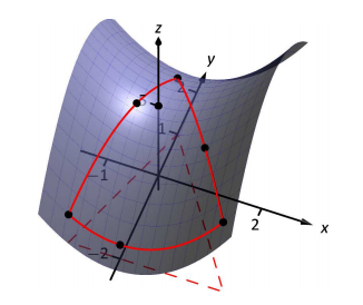
Figure \(\PageIndex{2}\): The surface of \(f\) along with important points along the boundary of \(S\) and the interior.
We have evaluated \(f\) at a total of \(7\) different places, all shown in Figure \(\PageIndex{2}\). We checked each vertex of the triangle twice, as each showed up as the endpoint of an interval twice. Of all the \(z\)-values found, the maximum is \(5.8\), found at \((1.2,-0.8)\); the minimum is \(1\), found at \((0,-2)\).
Notice that in this example we did not need to use the Second Partials Test to analyze the function's behavior at any critical points within the closed, bounded region. All we needed to do was evaluate the function at these critical points and then to find and evaluate the function at any critical points on the boundaries of this region. The largest output gives us the absolute maximum value of the function on the region, and the smallest output gives us the absolute minimum value of the function on the region.
Let's summarize the process we'll use for these problems.
Problem-Solving Strategy: Finding Absolute Maximum and Minimum Values on a Closed, Bounded Region
Let \(z=f(x,y)\) be a continuous function of two variables defined on a closed, bounded region \(D\), and assume \(f\) is differentiable on \(D\). To find the absolute maximum and minimum values of \(f\) on \(D\), do the following:
- Determine the critical points of \(f\) in \(D\).
- Calculate \(f\) at each of these critical points.
- Determine the maximum and minimum values of \(f\) on the boundary of its domain.
- The maximum and minimum values of \(f\) will occur at one of the values obtained in steps \(2\) and \(3\).
This portion of the text is entitled "Constrained Optimization'' because we want to optimize a function (i.e., find its maximum and/or minimum values) subject to a constraint -- limits on which input points are considered. In the previous example, we constrained ourselves by considering a function only within the boundary of a triangle. This was largely arbitrary; the function and the boundary were chosen just as an example, with no real "meaning'' behind the function or the chosen constraint.
However, solving constrained optimization problems is a very important topic in applied mathematics. The techniques developed here are the basis for solving larger problems, where more than two variables are involved.
We illustrate the technique again with a classic problem.
Example \(\PageIndex{3}\): Constrained Optimization of a Package
The U.S. Postal Service states that the girth plus the length of Standard Post Package must not exceed 130''. Given a rectangular box, the "length'' is the longest side, and the "girth'' is twice the sum of the width and the height.
Given a rectangular box where the width and height are equal, what are the dimensions of the box that give the maximum volume subject to the constraint of the size of a Standard Post Package?
SOLUTION
Let \(w\), \(h\) and \(\ell\) denote the width, height and length of a rectangular box; we assume here that \(w=h\). The girth is then \(2(w+h) = 4w\). The volume of the box is \(V(w,\ell) = wh\ell = w^2\ell\). We wish to maximize this volume subject to the constraint \(4w+\ell\leq 130\), or \(\ell\leq 130-4w\). (Common sense also indicates that \(\ell>0, w>0\).)
We begin by finding the critical values of \(V\). We find that \(V_w(w,\ell) = 2w\ell\) and \(V_\ell(w,\ell) = w^2\); these are simultaneously 0 only at \((0,0)\). This gives a volume of 0, so we can ignore this critical point.
We now consider the volume along the constraint \(\ell=130-4w.\) Along this line, we have:
\[V(w,\ell) = V(w,130-4w) = w^2(130-4w) = 130w^2-4w^3 = V_1(w).\]
The constraint restricts \(w\) to the interval \([0,32.5]\), as indicated in the figure. Thus we want to maximize \(V_1\) on \([0,32.5]\).
Finding the critical values of \(V_1\), we take the derivative and set it equal to \(0\):
\[V\,'_1(w) = 260w-12w^2 = 0 \quad \Rightarrow \quad w(260-12w)= 0 \quad \Rightarrow \quad w=0\;\text{ or }\; w=\tfrac{260}{12}\approx 21.67.\]
We found two critical values: when \(w=0\) and when \(w=21.67\). We again ignore the \(w=0\) solution. The maximum volume, subject to the constraint, comes at \(w=h=21.67\), \(\ell = 130-4(21.6) =43.33.\) This gives a maximum volume of \(V(21.67,43.33) \approx 19,408\) in\(^3\).
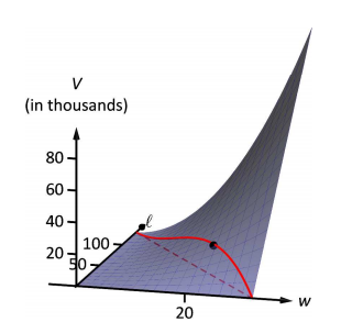
Figure \(\PageIndex{3}\): Graphing the volume of a box with girth \(4w\) and length \(\ell\), subject to a size constraint.
The volume function \(V(w,\ell)\) is shown in Figure \(\PageIndex{3}\) along with the constraint \(\ell = 130-4w\). As done previously, the constraint is drawn dashed in the \(xy\)-plane and also projected up onto the surface of the function. The point where the volume is maximized is indicated.
Finding the maximum and minimum values of \(f\) on the boundary of \(D\) can be challenging. If the boundary is a rectangle or set of straight lines, then it is possible to parameterize the line segments and determine the maxima on each of these segments, as seen in Example \(\PageIndex{1}\). The same approach can be used for other shapes such as circles and ellipses.
If the boundary of the region \(D\) is a more complicated curve defined by a function \(g(x,y)=c\) for some constant \(c\), and the first-order partial derivatives of \(g\) exist, then the method of Lagrange multipliers can prove useful for determining the extrema of \(f\) on the boundary.
Before we get to the method of Lagrange Multipliers (in the next section), let's consider a few additional examples of doing constrained optimization problems in this way.
Example \(\PageIndex{4}\): Finding Absolute Extrema
Use the problem-solving strategy for finding absolute extrema of a function to determine the absolute extrema of each of the following functions:
- \(f(x,y)=x^2−2xy+4y^2−4x−2y+24\) on the domain defined by \(0≤x≤4\) and \(0≤y≤2\)
- \(g(x,y)=x^2+y^2+4x−6y\) on the domain defined by \(x^2+y^2≤16\)
Solution:
a. Using the problem-solving strategy, step \(1\) involves finding the critical points of \(f\) on its domain. Therefore, we first calculate \(f_x(x,y)\) and \(f_y(x,y)\), then set them each equal to zero:
\[\begin{align*} f_x(x,y)&=2x−2y−4 \\f_y(x,y)&=−2x+8y−2. \end{align*}\]
Setting them equal to zero yields the system of equations
\[\begin{align*} 2x−2y−4&=0\\−2x+8y−2&=0. \end{align*}\]
The solution to this system is \(x=3\) and \(y=1\). Therefore \((3,1)\) is a critical point of \(f\). Calculating \(f(3,1)\) gives \(f(3,1)=17.\)
The next step involves finding the extrema of \(f\) on the boundary of its domain. The boundary of its domain consists of four line segments as shown in the following graph:
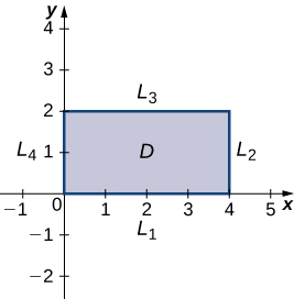
\(L_1\) is the line segment connecting \((0,0)\) and \((4,0)\), and it can be parameterized by the equations \(x(t)=t,y(t)=0\) for \(0≤t≤4\). Define \(g(t)=f\big(x(t),y(t)\big)\). This gives \(g(t)=t^2−4t+24\). Differentiating \(g\) leads to \(g′(t)=2t−4.\) Therefore, \(g\) has a critical value at \(t=2\), which corresponds to the point \((2,0)\). Calculating \(f(2,0)\) gives the \(z\)-value \(20\).
\(L_2\) is the line segment connecting \((4,0)\) and \((4,2)\), and it can be parameterized by the equations \(x(t)=4,y(t)=t\) for \(0≤t≤2.\) Again, define \(g(t)=f\big(x(t),y(t)\big).\) This gives \(g(t)=4t^2−10t+24.\) Then, \(g′(t)=8t−10\). g has a critical value at \(t=\frac{5}{4}\), which corresponds to the point \(\left(4,\frac{5}{4}\right).\) Calculating \(f\left(4,\frac{5}{4}\right)\) gives the \(z\)-value \(17.75\).
\(L_3\) is the line segment connecting \((0,2)\) and \((4,2)\), and it can be parameterized by the equations \(x(t)=t,y(t)=2\) for \(0≤t≤4.\) Again, define \(g(t)=f\big(x(t),y(t)\big).\) This gives \(g(t)=t^2−8t+36.\) The critical value corresponds to the point \((4,2).\) So, calculating \(f(4,2)\) gives the \(z\)-value \(20\).
\(L_4\) is the line segment connecting \((0,0)\) and \((0,2)\), and it can be parameterized by the equations \(x(t)=0,y(t)=t\) for \(0≤t≤2.\) This time, \(g(t)=4t^2−2t+24\) and the critical value \(t=\frac{1}{4}\) correspond to the point \(\left(0,\frac{1}{4}\right)\). Calculating \(f\left(0,\frac{1}{4}\right)\) gives the \(z\)-value \(23.75.\)
We also need to find the values of \(f(x,y)\) at the corners of its domain. These corners are located at \((0,0),(4,0),(4,2)\) and \((0,2)\):
\[\begin{align*} f(0,0)&=(0)^2−2(0)(0)+4(0)^2−4(0)−2(0)+24=24 \\f(4,0)&=(4)^2−2(4)(0)+4(0)^2−4(4)−2(0)+24=24 \\ f(4,2)&=(4)^2−2(4)(2)+4(2)^2−4(4)−2(2)+24=20\\ f(0,2)&=(0)^2−2(0)(2)+4(2)^2−4(0)−2(2)+24=36. \end{align*}\]
The absolute maximum value is \(36\), which occurs at \((0,2)\), and the global minimum value is \(20\), which occurs at both \((4,2)\) and \((2,0)\) as shown in the following figure.

b. Using the problem-solving strategy, step \(1\) involves finding the critical points of \(g\) on its domain. Therefore, we first calculate \(g_x(x,y)\) and \(g_y(x,y)\), then set them each equal to zero:
\[\begin{align*} g_x(x,y)&=2x+4 \\ g_y(x,y)&=2y−6. \end{align*}\]
Setting them equal to zero yields the system of equations
\[\begin{align*} 2x+4&=0 \\ 2y−6&=0. \end{align*}\]
The solution to this system is \(x=−2\) and \(y=3\). Therefore, \((−2,3)\) is a critical point of \(g\). Calculating \(g(−2,3),\) we get
\[g(−2,3)=(−2)^2+3^2+4(−2)−6(3)=4+9−8−18=−13. \nonumber\]
The next step involves finding the extrema of \(g\) on the boundary of its domain. The boundary of its domain consists of a circle of radius \(4\) centered at the origin as shown in the following graph.
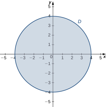
The boundary of the domain of g can be parameterized using the functions \(x(t)=4\cos t,\, y(t)=4\sin t\) for \(0≤t≤2π\). Define \(h(t)=g\big(x(t),y(t)\big):\)
\[\begin{align*} h(t)&=g\big(x(t),y(t)\big) \\&=(4\cos t)^2+(4\sin t)^2+4(4\cos t)−6(4\sin t) \\ &=16\cos^2t+16\sin^2t+16\cos t−24\sin t\\&=16+16\cos t−24\sin t. \end{align*}\]
Setting \(h′(t)=0\) leads to
\[\begin{align*} −16\sin t−24\cos t&=0 \\ −16\sin t&=24\cos t\\\dfrac{−16\sin t}{−16\cos t}&=\dfrac{24\cos t}{−16\cos t} \\\tan t&=−\dfrac{4}{3}. \end{align*}\]
\[\begin{align*} −16\sin t−24\cos t&=0 \\ −16\sin t&=24\cos t\\\dfrac{−16\sin t}{−16\cos t}&=\dfrac{24\cos t}{−16\cos t} \\\tan t&=−\dfrac{3}{2}. \end{align*}\]
This equation has two solutions over the interval \(0≤t≤2π\). One is \(t=π−\arctan (\frac{3}{2})\) and the other is \(t=2π−\arctan (\frac{3}{2})\). For the first angle,
\[\begin{align*} \sin t&=\sin(π−\arctan(\tfrac{3}{2}))=\sin (\arctan (\tfrac{3}{2}))=\dfrac{3\sqrt{13}}{13} \\ \cos t&=\cos (π−\arctan (\tfrac{3}{2}))=−\cos (\arctan (\tfrac{3}{2}))=−\dfrac{2\sqrt{13}}{13}. \end{align*}\]
Therefore, \(x(t)=4\cos t=−\frac{8\sqrt{13}}{13}\) and \(y(t)=4\sin t=\frac{12\sqrt{13}}{13}\), so \(\left(−\frac{8\sqrt{13}}{13},\frac{12\sqrt{13}}{13}\right)\) is a critical point on the boundary and
\[\begin{align*} g\left(−\tfrac{8\sqrt{13}}{13},\tfrac{12\sqrt{13}}{13}\right)&=\left(−\tfrac{8\sqrt{13}}{13}\right)^2+\left(\tfrac{12\sqrt{13}}{13}\right)^2+4\left(−\tfrac{8\sqrt{13}}{13}\right)−6\left(\tfrac{12}{\sqrt{13}}{13}\right) \\&=\frac{144}{13}+\frac{64}{13}−\frac{32\sqrt{13}}{13}−\frac{72\sqrt{13}}{13} \\&=\frac{208−104\sqrt{13}}{13}≈−12.844. \end{align*}\]
For the second angle,
\[\begin{align*} \sin t&=\sin (2π−\arctan (\tfrac{3}{2}))=−\sin (\arctan (\tfrac{3}{2}))=−\dfrac{3\sqrt{13}}{13} \\ \cos t&=\cos (2π−\arctan (\tfrac{3}{2}))=\cos (\arctan (\tfrac{3}{2}))=\dfrac{2\sqrt{13}}{13}. \end{align*}\]
Therefore, \(x(t)=4\cos t=\frac{8\sqrt{13}}{13}\) and \(y(t)=4\sin t=−\frac{12\sqrt{13}}{13}\), so \(\left(\frac{8\sqrt{13}}{13},−\frac{12\sqrt{13}}{13}\right)\) is a critical point on the boundary and
\[\begin{align*} g\left(\tfrac{8\sqrt{13}}{13},−\tfrac{12\sqrt{13}}{13}\right)&=\left(\tfrac{8\sqrt{13}}{13}\right)^2+\left(−\tfrac{12\sqrt{13}}{13}\right)^2+4\left(\tfrac{8\sqrt{13}}{13}\right)−6\left(−\tfrac{12\sqrt{13}}{13}\right) \\ &=\dfrac{144}{13}+\dfrac{64}{13}+\dfrac{32\sqrt{13}}{13}+\dfrac{72\sqrt{13}}{13}\\ &=\dfrac{208+104\sqrt{13}}{13}≈44.844. \end{align*}\]
The absolute minimum of g is \(−13,\) which is attained at the point \((−2,3)\), which is an interior point of D. The absolute maximum of g is approximately equal to 44.844, which is attained at the boundary point \(\left(\frac{8\sqrt{13}}{13},−\frac{12\sqrt{13}}{13}\right)\). These are the absolute extrema of g on D as shown in the following figure.
Exercise \(\PageIndex{1}\)
Use the problem-solving strategy for finding absolute extrema of a function to find the absolute extrema of the function
\[f(x,y)=4x^2−2xy+6y^2−8x+2y+3 \nonumber\]
on the domain defined by \(0≤x≤2\) and \(−1≤y≤3.\)
- Hint
-
Calculate \(f_x(x,y)\) and \(f_y(x,y)\), and set them equal to zero. Then, calculate \(f\) for each critical point and find the extrema of \(f\) on the boundary of \(D\).
- Answer
-
The absolute minimum occurs at \((1,0): f(1,0)=−1.\)
The absolute maximum occurs at \((0,3): f(0,3)=63.\)
Example \(\PageIndex{5}\): Profitable Golf Balls
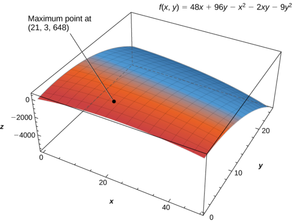
Pro-\(T\) company has developed a profit model that depends on the number \(x\) of golf balls sold per month (measured in thousands), and the number of hours per month of advertising \(y\), according to the function
\[ z=f(x,y)=48x+96y−x^2−2xy−9y^2,\]
where \(z\) is measured in thousands of dollars. The maximum number of golf balls that can be produced and sold is \(50,000\), and the maximum number of hours of advertising that can be purchased is \(25\). Find the values of \(x\) and \(y\) that maximize profit, and find the maximum profit.
Solution
Using the problem-solving strategy, step \(1\) involves finding the critical points of \(f\) on its domain. Therefore, we first calculate \(f_x(x,y)\) and \(f_y(x,y),\) then set them each equal to zero:
\[\begin{align*} f_x(x,y)&=48−2x−2y \\ f_y(x,y)&=96−2x−18y. \end{align*}\]
Setting them equal to zero yields the system of equations
\[\begin{align*} 48−2x−2y&=0 \\ 96−2x−18y&=0. \end{align*}\]
The solution to this system is \(x=21\) and \(y=3\). Therefore \((21,3)\) is a critical point of \(f\). Calculating \(f(21,3)\) gives \(f(21,3)=48(21)+96(3)−21^2−2(21)(3)−9(3)^2=648.\)
The domain of this function is \(0≤x≤50\) and \(0≤y≤25\) as shown in the following graph.
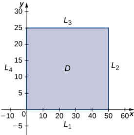
\(L_1\) is the line segment connecting \((0,0)\) and \((50,0),\) and it can be parameterized by the equations \(x(t)=t,y(t)=0\) for \(0≤t≤50.\) We then define \(g(t)=f(x(t),y(t)):\)
\[\begin{align*} g(t)&=f(x(t),y(t)) \\ &=f(t,0)\\ &=48t+96(0)−y^2−2(t)(0)−9(0)^2\\ &=48t−t^2. \end{align*}\]
Setting \(g′(t)=0\) yields the critical point \(t=24,\) which corresponds to the point \((24,0)\) in the domain of \(f\). Calculating \(f(24,0)\) gives \(576.\)
\(L_2\) is the line segment connecting and \((50,25)\), and it can be parameterized by the equations \(x(t)=50,y(t)=t\) for \(0≤t≤25\). Once again, we define \(g(t)=f\big(x(t),y(t)\big):\)
\[\begin{align*} g(t)&=f\big(x(t),y(t)\big)\\ &=f(50,t)\\&=48(50)+96t−50^2−2(50)t−9t^2 \\&=−9t^2−4t−100. \end{align*}\]
This function has a critical point at \(t =−\frac{2}{9}\), which corresponds to the point \((50,−29)\). This point is not in the domain of \(f\).
\(L_3\) is the line segment connecting \((0,25)\) and \((50,25)\), and it can be parameterized by the equations \(x(t)=t,y(t)=25\) for \(0≤t≤50\). We define \(g(t)=f\big(x(t),y(t)\big)\):
\[\begin{align*} g(t)&=f\big(x(t),y(t)\big)\\&=f(t,25) \\&=48t+96(25)−t^2−2t(25)−9(25^2) \\&=−t^2−2t−3225. \end{align*}\]
This function has a critical point at \(t=−1\), which corresponds to the point \((−1,25),\) which is not in the domain.
\(L_4\) is the line segment connecting \((0,0)\) to \((0,25)\), and it can be parameterized by the equations \(x(t)=0,y(t)=t\) for \(0≤t≤25\). We define \(g(t)=f\big(x(t),y(t)\big)\):
\[\begin{align*} g(t)&=f\big(x(t),y(t)\big) \\&=f(0,t) \\ &=48(0)+96t−(0)^2−2(0)t−9t^2 \\ &=96t−t^2. \end{align*}\]
This function has a critical point at \(t=\frac{16}{3}\), which corresponds to the point \(\left(0,\frac{16}{3}\right)\), which is on the boundary of the domain. Calculating \(f\left(0,\frac{16}{3}\right)\) gives \(256\).
We also need to find the values of \(f(x,y)\) at the corners of its domain. These corners are located at \((0,0),(50,0),(50,25)\) and \((0,25)\):
\[\begin{align*} f(0,0)&=48(0)+96(0)−(0)^2−2(0)(0)−9(0)^2=0\\f(50,0)&=48(50)+96(0)−(50)^2−2(50)(0)−9(0)^2=−100 \\f(50,25)&=48(50)+96(25)−(50)^2−2(50)(25)−9(25)^2=−5825 \\ f(0,25)&=48(0)+96(25)−(0)^2−2(0)(25)−9(25)^2=−3225. \end{align*}\]
The maximum critical value is \(648\), which occurs at \((21,3)\). Therefore, a maximum profit of \($648,000\) is realized when \(21,000\) golf balls are sold and \(3\) hours of advertising are purchased per month as shown in the following figure.
It is hard to overemphasize the importance of optimization. In "the real world,'' we routinely seek to make something better. By expressing the something as a mathematical function, "making something better'' means to "optimize some function.''
The techniques shown here are only the beginning of a very important field. But be aware that many functions that we will want to optimize are incredibly complex, making the step to "find the gradient, set it equal to \(\vecs 0\), and find all points that make this true'' highly nontrivial. Mastery of the principles on simpler problems here is key to being able to tackle these more complicated problems.
The Method of Least Squares Regression
Our world is full of data, and to interpret and extrapolate based on this data, we often try to find a function to model this data in a particular situation. You've likely heard about a line of best fit, also known as a least squares regression line. This linear model, in the form \(f(x) = ax + b\), assumes the value of the output changes at a roughly constant rate with respect to the input, i.e., that these values are related linearly. And for many situations this linear model gives us a powerful way to make predictions about the value of the function's output for inputs other than those in the data we collected. For other situations, like most population models, a linear model is not sufficient, and we need to find a quadratic, cubic, exponential, logistic, or trigonometric model (or possibly something else).
Consider the data points given in the table below. Figures \(\PageIndex{11}\) - \(\PageIndex{14}\) show various best fit regression models for this data.
\( \qquad \begin{array}{c | c}
x & y \\ \hline
2 & 1 \\
4 & 2 \\
6 & 4 \\
8 & 7
\end{array}
\)
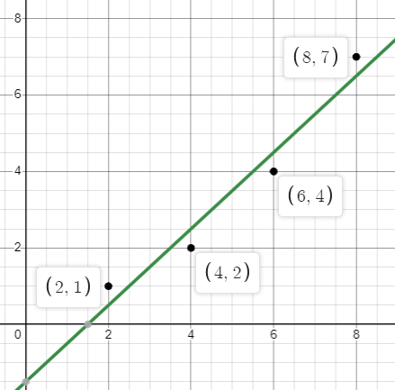
Figure \(\PageIndex{11}\): Linear model
\(y = x - 1.5 \)

Figure \(\PageIndex{12}\): Quadratic model
\( y = 0.125x^2 - 0.25x + 1 \)

Figure \(\PageIndex{13}\): Exponential model
\( y = 0.6061 \cdot (1.359)^x \)

Figure \(\PageIndex{14}\): Logistic model
\( y = \dfrac{18.31}{1 + 39.67 e^{-0.4002 x}} \)
One way to measure how well a particular model \( y = f(x) \) fits a given set of data points \(\big\{(x_1, y_1), (x_2, y_2), (x_3, y_3), ..., (x_n, y_n)\big\}\) is to consider the squares of the differences between the values given by the model and the actual \(y\)-values of the data points.

The differences (or errors), \(d_i = f(x_i) - y_i\), are squared and added up so that all errors are considered in the measure of how well the model "fits" the data. This sum of the squared errors is given by
\[S = \sum_{i=1}^n \big( f(x_i) - y_i \big)^2 \nonumber\]
Squaring the errors in this sum also tends to magnify the weight of larger errors and minimize the weight of small errors in the measurement of how well the model fits the data.
Note that \(S\) is a function of the constant parameters in the particular model \( y = f(x) \). For example, if we desire a linear model, then \( f(x) = a x + b\), and
\[\begin{align*} S(a, b) &= \sum_{i=1}^n \big( f(x_i) - y_i \big)^2 \\ &= \sum_{i=1}^n \big( a x_i + b - y_i \big)^2 \end{align*} \]
To obtain the best fit version of the model, we will seek the values of the constant parameters in the model (\(a\) and \(b\) in the linear model) that give us the minimum value of this sum of the squared errors function \(S\) for the given set of data points.
When calculating a line of best fit in previous classes, you were likely either given the formulas for the coefficients or shown how to use features on your calculator or other device to find them.
Using our understanding of the optimization of functions of multiple variables in this class, we are now able to derive the formulas for these coefficients directly. In fact, we can use the same methods to determine the constant parameters needed to form a best fit model of any kind (quadratic, cubic, exponential, logistic, sine, cosine, etc), although these can be a bit more difficult to work out than the linear case.
The least squares regression line (or line of best fit) for the data points \(\big\{(x_1, y_1), (x_2, y_2), (x_3, y_3), ..., (x_n, y_n)\big\}\) is given by the formula
\[f(x) = ax + b \nonumber\]
where
\[ a = \dfrac{\displaystyle {n \dsum_{i=1}^n x_i y_i - \dsum_{i=1}^n x_i \dsum_{i=1}^n y_i}}{\displaystyle{n\dsum_{i=1}^n {x_i}^2 - \left( \dsum_{i=1}^n x_i \right)^2}} \qquad \text{and} \qquad b = \tfrac{1}{n}\left(\dsum_{i=1}^n y_i - a\dsum_{i=1}^n x_i \right). \nonumber\]
Proof (part 1): To obtain a line that best fits the data points we need to minimize the sum of the squared errors for this model. This is a function of the two variables \(a\) and \(b\) as shown below. Note that the \(x_i\) and \(y_i\) are numbers in this function and are not the variables.
\[ S(a, b) = \sum_{i=1}^n \big( a x_i + b - y_i \big)^2 \nonumber \]
To minimize this function of the two variables \(a\) and \(b\), we need to determine the critical point(s) of this function. Let's start by stating the partial derivatives of \(S\) with respect to \(a\) and \(b\) and simplifying them so that the sums only include the numerical coordinates from the data points.
\[ \begin{align*} S_a(a, b) &= \sum_{i=1}^n 2x_i\big( a x_i + b - y_i \big) \\
&= \sum_{i=1}^n \big( 2a {x_i}^2 + 2b x_i - 2x_i y_i \big) \\
&= \sum_{i=1}^n 2a {x_i}^2 + \sum_{i=1}^n 2b x_i - \sum_{i=1}^n 2x_i y_i \\
&= 2a \sum_{i=1}^n {x_i}^2 + 2b \sum_{i=1}^n x_i - 2 \sum_{i=1}^n x_i y_i \end{align*} \]
\[ \begin{align*} S_b(a, b) &= \sum_{i=1}^n 2 \big( a x_i + b - y_i \big) \\
&= \sum_{i=1}^n \big( 2a x_i + 2b - 2 y_i \big) \\
&= \sum_{i=1}^n 2a x_i + \sum_{i=1}^n 2b - \sum_{i=1}^n 2 y_i \\
&= 2a \sum_{i=1}^n x_i + 2b \sum_{i=1}^n 1 - 2 \sum_{i=1}^n y_i \\
&= 2a \sum_{i=1}^n x_i + 2b n - 2 \sum_{i=1}^n y_i \end{align*} \]
Next we set these partial derivatives equal to \(0\) and solve the resulting system of equations.
Set \(\displaystyle 2a \dsum_{i=1}^n {x_i}^2 + 2b \dsum_{i=1}^n x_i - 2 \dsum_{i=1}^n x_i y_i = 0 \),
and \( \displaystyle 2a \dsum_{i=1}^n x_i + 2b n - 2 \dsum_{i=1}^n y_i = 0 \).
Since the linear case is simple enough to make this process straightforward, we can use substitution to actually solve this system for \(a\) and \(b\). Solving the second equation for \(b\) gives us
\(\qquad \displaystyle 2bn = 2 \dsum_{i=1}^n y_i - 2a \dsum_{i=1}^n x_i \)
\(\qquad \displaystyle \boxed{b = \tfrac{1}{n}\left(\dsum_{i=1}^n y_i - a\dsum_{i=1}^n x_i \right).} \)
We now substitute this expression into the first equation for \(b\).
\(\qquad \displaystyle 2a \dsum_{i=1}^n {x_i}^2 + 2\left[\tfrac{1}{n}\left(\dsum_{i=1}^n y_i - a\dsum_{i=1}^n x_i \right)\right] \dsum_{i=1}^n x_i - 2 \dsum_{i=1}^n x_i y_i = 0 \)
Multiplying this equation through by \(n\) and dividing out the \(2\) yields
\(\qquad \displaystyle an \dsum_{i=1}^n {x_i}^2 + \left[\dsum_{i=1}^n y_i - a\dsum_{i=1}^n x_i \right] \dsum_{i=1}^n x_i - n \dsum_{i=1}^n x_i y_i = 0. \)
Simplifying,
\(\qquad \displaystyle an \dsum_{i=1}^n {x_i}^2 + \dsum_{i=1}^n x_i \dsum_{i=1}^n y_i - a\dsum_{i=1}^n x_i \sum_{i=1}^n x_i - n \dsum_{i=1}^n x_i y_i = 0. \)
Next we isolate the terms containing \(a\) on the left side of the equation, moving the other two terms to the right side of the equation.
\(\qquad \displaystyle an \dsum_{i=1}^n {x_i}^2 - a\left(\dsum_{i=1}^n x_i\right)^2 = n \dsum_{i=1}^n x_i y_i - \dsum_{i=1}^n x_i \dsum_{i=1}^n y_i. \)
Factoring out the \(a\),
\(\qquad \displaystyle a\left( n \dsum_{i=1}^n {x_i}^2 - \left(\dsum_{i=1}^n x_i\right)^2\right) = n \dsum_{i=1}^n x_i y_i - \dsum_{i=1}^n x_i \dsum_{i=1}^n y_i. \)
Finally, we solve for \(a\) to obtain
\( \qquad \displaystyle \boxed{a = \dfrac{\displaystyle {n \dsum_{i=1}^n x_i y_i - \dsum_{i=1}^n x_i \dsum_{i=1}^n y_i}}{\displaystyle{n\dsum_{i=1}^n {x_i}^2 - \left( \dsum_{i=1}^n x_i \right)^2}}.} \qquad \)
\(\qquad \qquad \qquad \qquad \qquad \qquad \qquad \qquad \blacksquare \qquad\text{QED} \)
Thus we have found formulas for the coordinates of the single critical point of the sum of squared errors function for the linear model, i.e.,
\(\qquad \displaystyle S(a, b) = \dsum_{i=1}^n \big( a x_i + b - y_i \big)^2 \).
Proof (part 2): To prove that this linear model gives us a minimum of \(S\), we will need the Second Partials Test.
The second partials of \(S\) are
\[ \begin{align*} S_{aa}(a,b) &= \sum_{i=1}^n 2{x_i}^2 \\ S_{bb}(a,b) &= \sum_{i=1}^n 2 = 2n \\ S_{ab}(a,b) &= \sum_{i=1}^n 2 x_i. \end{align*}\]
Then the discriminant evaluated at the critical point \( (a, b) \) is
\[ \begin{align*} D(a, b) &= S_{aa}(a,b) S_{bb}(a,b) - \big[ S_{ab}(a,b) \big]^2 \\
&= 2n \sum_{i=1}^n 2{x_i}^2 - \left( 2 \sum_{i=1}^n x_i \right)^2 \\
&= 4n \sum_{i=1}^n {x_i}^2 - 4 \left( \sum_{i=1}^n x_i \right)^2 \\
&= 4\left[ n \sum_{i=1}^n {x_i}^2 - \left( \sum_{i=1}^n x_i \right)^2 \right]. \end{align*} \]
Now to prove that this discriminant is positive (and thus guarantees a local max or min) requires us to use the Cauchy-Schwarz Inequality. This part of the proof is non-trivial, but not too hard, if we don't worry about proving the Cauchy-Schwarz Inequality itself here.
The Cauchy-Schwarz Inequality guarantees
\[ \left(\sum_{i=1}^n a_i b_i\right)^2 \leq \left(\sum_{i=1}^n {a_i}^2 \right) \left(\sum_{i=1}^n {b_i}^2 \right)\nonumber\]
for any real-valued sequences \(a_i\) and \(b_i\), with equality only if these two sequences are dependent (e.g., if the terms were the same or some multiple of each other).
Here we choose \(a_i = 1\) and \(b_i = x_i\). Since these sequences are linearly independent, we will not have equality and substituting into the Cauchy-Schwarz Inequality gives us
\[ \left(\sum_{i=1}^n 1 \cdot x_i \right)^2 < \left(\sum_{i=1}^n {1}^2 \right) \left(\sum_{i=1}^n {x_i}^2 \right). \nonumber \]
Since \( \dsum_{i=1}^n 1 = n \), we have
\[ \left(\sum_{i=1}^n x_i \right)^2 < n \sum_{i=1}^n {x_i}^2. \nonumber\]
This result proves
\[D(a,b) = 4\left[ n \sum_{i=1}^n {x_i}^2 - \left( \sum_{i=1}^n x_i \right)^2 \right] > 0. \nonumber\]
Now, since it is clear that \(\displaystyle S_{aa}(a,b) = \dsum_{i=1}^n 2{x_i}^2 > 0 \), we know that \(S\) is concave up at the point \( (a, b) \) and thus has a relative minimum there. This concludes the proof that the parameters \(a\) and \(b\), as shown in Theorem
\[f(x) = ax + b. \qquad \qquad \qquad \blacksquare \qquad\text{QED} \nonumber \]
The linear case \(f(x)=ax+b\) is special in that it is simple enough to allow us to actually solve for the constant parameters \(a\) and \(b\) directly as formulas (as shown above in Theorem \(\PageIndex{2}\). For other best fit models we typically just obtain the system of equations needed to solve for the corresponding constant parameters that give us the critical point and minimum value of \(S\).
To leave the quadratic regression case for you to try as an exercise, let's consider a cubic best fit model here.
Determine the system of equations needed to determine the cubic best fit regression model of the form, \( f(x) = ax^3 + bx^2 + cx + d \), for a given set of data points, \(\big\{(x_1, y_1), (x_2, y_2), (x_3, y_3), ..., (x_n, y_n)\big\}\).
Solution
Here consider the sum of least squares function
\[ S(a, b, c, d) = \sum_{i=1}^n \big( a {x_i}^3 + b {x_i}^2 + c x_i + d - y_i \big)^2. \nonumber \]
To find the minimum value of this function (and the corresponding values of the parameters \(a, b, c,\) and \(d\) needed for the best fit cubic regression model), we need to find the critical point of this function. (Yes, even for a function of four variables!) To begin this process, we find the first partial derivatives of this function with respect to each of the parameters \(a, b, c,\) and \(d\).
\[ \begin{align*} S_a(a, b, c, d) &= 2 \sum_{i=1}^n {x_i}^3 \big( a {x_i}^3 + b {x_i}^2 + c x_i + d - y_i \big) \\
S_b(a, b, c, d) &= 2 \sum_{i=1}^n {x_i}^2 \big( a {x_i}^3 + b {x_i}^2 + c x_i + d - y_i \big) \\
S_c(a, b, c, d) &= 2 \sum_{i=1}^n x_i \big( a {x_i}^3 + b {x_i}^2 + c x_i + d - y_i \big) \\
S_d(a, b, c, d) &= 2 \sum_{i=1}^n \big( a {x_i}^3 + b {x_i}^2 + c x_i + d - y_i \big) \end{align*} \]
Now we set these partials equal to \(0\), divide out the 2 from each, and split the terms into separate sums. We also factor out the \(a, b, c,\) and \(d\) which don't change as the index changes.
\[ \begin{align*} a \sum_{i=1}^n {x_i}^6 + b \sum_{i=1}^n {x_i}^5 + c \sum_{i=1}^n {x_i}^4 + d\sum_{i=1}^n {x_i}^3 - \sum_{i=1}^n {x_i}^3 y_i = 0 \\
a \sum_{i=1}^n {x_i}^5 + b \sum_{i=1}^n {x_i}^4 + c \sum_{i=1}^n {x_i}^3 + d\sum_{i=1}^n {x_i}^2 - \sum_{i=1}^n {x_i}^2 y_i = 0 \\
a \sum_{i=1}^n {x_i}^4 + b \sum_{i=1}^n {x_i}^3 + c \sum_{i=1}^n {x_i}^2 + d\sum_{i=1}^n x_i - \sum_{i=1}^n x_i y_i = 0 \\
a \sum_{i=1}^n {x_i}^3 + b \sum_{i=1}^n {x_i}^2 + c \sum_{i=1}^n x_i + d\sum_{i=1}^n 1 - \sum_{i=1}^n y_i = 0 \\ \end{align*} \]
This system of equations can be rewritten by moving the negative terms to the right side of the equation. We'll also emphasize the coefficients and variables and replace \( \dsum_{i=1}^n 1 \) with \(n\).
\[ \begin{align*} \left( \sum_{i=1}^n {x_i}^6 \right)a + \left( \sum_{i=1}^n {x_i}^5 \right) b + \left( \sum_{i=1}^n {x_i}^4 \right) c +\left(\sum_{i=1}^n {x_i}^3 \right) d = \sum_{i=1}^n {x_i}^3 y_i \\
\left(\sum_{i=1}^n {x_i}^5 \right) a + \left( \sum_{i=1}^n {x_i}^4 \right) b + \left( \sum_{i=1}^n {x_i}^3 \right) c + \left(\sum_{i=1}^n {x_i}^2 \right) d = \sum_{i=1}^n {x_i}^2 y_i \\
\left(\sum_{i=1}^n {x_i}^4 \right) a +\left( \sum_{i=1}^n {x_i}^3 \right) b + \left( \sum_{i=1}^n {x_i}^2 \right) c + \left( \sum_{i=1}^n x_i \right) d = \sum_{i=1}^n x_i y_i \\
\left( \sum_{i=1}^n {x_i}^3 \right) a + \left( \sum_{i=1}^n {x_i}^2 \right) b +\left( \sum_{i=1}^n x_i \right) c + nd = \sum_{i=1}^n y_i \\ \end{align*} \]
This is a system of four linear equations with the four variables \(a, b, c,\) and \(d\). To solve for the values of these parameters that would give us the best fit cubic regression model, we would need to solve this system using the given data points. We would first evaluate each of the sums using the \(x\)- and \(y\)-coordinates of the data points and place these numerical coefficients into the equations. We would then only need to solve the resulting system of linear equations.
Let's now use this process to find the best fit cubic regression model for a set of data points.
a. Find the best fit cubic regression model of the form, \( f(x) = ax^3 + bx^2 + cx + d \), for the set of data points below.
\(\qquad \begin{array}{c | c}
x & y \\ \hline
1 & 1 \\
4 & 3 \\
6 & 4 \\
8 & 7 \\
9 & 6
\end{array}
\)
b. Determine the actual sum of the squared errors for this cubic model and these data points.
Solution
a. First we need to calculate each of the sums that appear in the system of linear equations we derived in Example \(\PageIndex{6}\).Note first that since we have five points, \(n = 5\).
\[ \begin{align*} \sum_{i=1}^5 {x_i}^6 &= 1^6 + 4^6 + 6^6 + 8^6 + 9^6 = 844338 & & \sum_{i=1}^5 {x_i}^3 y_i = 1^3(1) + 4^3(3)+6^3(4)+8^3(7) + 9^3(6) = 9015\\
\sum_{i=1}^5 {x_i}^5 &= 1^5 + 4^5 + 6^5 + 8^5 + 9^5 = 100618 & & \sum_{i=1}^5 {x_i}^2 y_i = 1^2(1) + 4^2(3)+6^2(4)+8^2(7) + 9^2(6) = 1127 \\
\sum_{i=1}^5 {x_i}^4 &= 1^4 + 4^4 + 6^4 + 8^4 + 9^4 = 12210 & & \sum_{i=1}^5 x_i y_i = 1(1) + 4(3) + 6(4) + 8(7) + 9(6) = 147\\
\sum_{i=1}^5 {x_i}^3 &= 1^3 + 4^3 + 6^3 + 8^3 + 9^3 = 1522 & & \sum_{i=1}^5 y_i =1 + 3 + 4 + 7 + 6 = 21 \\
\sum_{i=1}^5 {x_i}^2 &= 1^2 + 4^2 + 6^2 + 8^2 + 9^2 = 198 & & \sum_{i=1}^5 x_i = 1 + 4 + 6 + 8 + 9 = 28 \\
\end{align*} \]
Plugging these values into the system of equations from Example \(\PageIndex{6}\) gives us
\[ \begin{align*} &844338 a + 100618 b + 12210 c +1522 d = 9015 \\
&100618 a + 12210 b + 1522 c + 198 d = 1127 \\
&12210 a +1522 b + 198 c + 28 d = 147 \\
&1522 a + 198 b + 28 c + 5 d = 21 \\ \end{align*} \]
Solving this system by elimination (or using row-reduction in matrix form) gives us
\[ a = -0.0254167, \; b = 0.382981, \; c = -0.852949, \; d = 1.547308 \nonumber\]
which results in the following cubic best fit regression model for this set of data points:
\[ f(x) = -0.0254167 x^3 + 0.382981 x^2 - 0.852949x + 1.547308. \nonumber \]
See this best fit cubic regression model along with these data points in Figure \(\PageIndex{16}\) below.

b. Now that we have the model, let's consider what the errors are for each data point and calculate the sum of the squared errors. This is the absolute minimum value of the function
\[ S(a, b, c, d) = \sum_{i=1}^n \big( a {x_i}^3 + b {x_i}^2 + c x_i + d - y_i \big)^2. \nonumber \]
\[\begin{array}{|c|c|c|c|}\hline x_i & y_i & f(x_i) & \mbox{Error: }f(x_i)-y_i & \mbox{Squared Error: }\left( f(x_i)-y_i \right)^2 \\ \hline 1 & 1 & 1.0519231 & 0.0519231 & 0.002696 \\ 4 & 3 & 2.6365385 & -0.3634615 & 0.132104 \\ 6 & 4 & 4.7269231 & 0.7269231 & 0.528417 \\ 8 & 7 & 6.2211538 & -0.7788462 & 0.606601 \\ 9 & 6 & 6.3634615 & 0.3634615 & 0.132104 \\ \hline \end{array} \\ \mbox{Total Squared Error in }S \approx 1.401922 \nonumber\]
Contributors
- Edited, Mixed, and expanded by Paul Seeburger (Monroe Community College)
(Applications of Optimization - Approach 1 and Example \(\PageIndex{1}\))
(The Method of Least Squares Regression) Gregory Hartman (Virginia Military Institute). Contributions were made by Troy Siemers and Dimplekumar Chalishajar of VMI and Brian Heinold of Mount Saint Mary's University. This content is copyrighted by a Creative Commons Attribution - Noncommercial (BY-NC) License. http://www.apexcalculus.com/
(Examples \(\PageIndex{2}\) and \(\PageIndex{3}\) and some exposition at top and bottom of section.)Gilbert Strang (MIT) and Edwin “Jed” Herman (Harvey Mudd) with many contributing authors. This content by OpenStax is licensed with a CC-BY-SA-NC 4.0 license. Download for free at http://cnx.org.
(Examples \(\PageIndex{4}\) and \(\PageIndex{5}\) and Exercise \(\PageIndex{1}\).)