4.5: Optimization

How do we use calculus to make decisions? If we’re trying to find the best allocation of time between different tasks, or if we’re trying to construct some object with limited resources, or if we’re trying to find some other solution to the question, “How do we make the best/most/maximum/minimum of...” then we can think about translating these to a calculus context.

Optimization problems are some of the clearest application of calculus concepts to applied problems from any industry or field. While there certainly aren’t teams of calculus experts in every office waiting for these kinds of problems to arrive, these problems are routinely solved using calculus, either done by computer software or coming from calculus experts who make sweeping recommendations across a whole field or some other source.

Optimization Framework

We’ll start this discussion with a small example. This is not an example that shows up in “real life,” but will be helpful to build a strategy for approaching these problems.

Here’s our problem:

Example \(\PageIndex{1}\)

Find two numbers that add to get 14 but give the largest possible product.

That’s it. That’s the problem. It’s not super interesting, right? Let’s think about how we’ll solve it.

Solution

Solution 1.

First, we want to think about our two numbers. We’ll need variable names for these. You can use whatever letters you’d like here: I’m going to be boring and pick \(a\) and \(b\) as the names of my two numbers. What do we know about \(a\) and \(b\)?

The first thing that we know is that \(a+b = 14\). This isn’t a huge amount of information, but it does provide us with a nice connection between our numbers. If we know what one number is, then we automatically know the second one: if one number is 4, then the other number is whatever we need to add to 4 to get 14.

We also know that we’re interested in the product: \(P = ab\). We don’t, currently, know anything about this product other than the fact that we want it to be large. Ok so automatically, we know that both \(a\) and \(b\) need to be positive: if we had one number that was positive (like 15) and one number that was negative (like −1), then the product will be negative, and even though they add to 14, we are not going to get a big product.

So we know that for both of these numbers \(a, b \geq 0\). This doesn’t seem like a lot of information, but we can put it all together really nicely. For instance, I can manipulate the fact that these two numbers add to get 14 into an equation that tells me what the value of one number is based on the other:

\[a+b=14 \longrightarrow b=14-a \nonumber \]

I can also write my product as an actual function of a single variable:

\[P=a b \longrightarrow P(a)=a(\underbrace{14-a}_b) \nonumber \]

Lastly, I actually know a domain for this function: we know that \(a \geq 0\), but since \(b \geq 0\), then \(a \leq 14\). We can’t have a number larger than 14, since the other number would be negative.

Aside.

I just said that we can’t have a negative product, but nothing in this problem says that. We just know that a negative product will be small. But we don’t have to limit each number to be between 0 and 14. We could just allow them to be bigger than 14 (and thus also allowed to be smaller than 0) and we’ll just get a bunch of negative products that aren’t the maximum one. Oh well!

We are making a similar choice by including the pair 0 and 14 as a possibility. Do we really think that this could give us the biggest product? NO! The product is 0! But it’s maybe convenient to have a closed interval as the domain of this function, so why not?

All along the way, we’re making choices that guide how we think about this problem. In real life, we’ll do the same thing. The only difference is that the choices that we make about what are reasonable values for our inputs to take on are more meaningful, since those inputs represent real things. We have to take these choices seriously.

Ok, so we have a function representing the product, \(P(a) = a(14 − a)\) and a domain for that function, [0, 14], and we know we want to find the maximum for it. This is a calculus problem that we can actually do! Take a moment to do it.

Solution 2.

\[\begin{aligned}
P(a) & =14 a-a^2 \\
P^{\prime}(a) & =14-2 a
\end{aligned} \nonumber \]

Now we can find the critical points.

\[\begin{aligned}
P^{\prime}(a) & =0 \\
14-2 a & =0 \\
-2 a & =-14 \\
a & =7
\end{aligned} \nonumber \]

We also know that the ending points at \(a = 0\) and \(a = 14\) are critical, since the derivative cannot exist.

There is a point on the product function when \(a = 7\) where we have a horizontal tangent line. Does this represent a maximum or a minimum? We have some options for how to do this:

1. FDT:

   \(a\)	[0, 7)	7	(7, 14]
   \(P^{\prime}\)	\(\oplus\)	0	\(\ominus\)
   \(P\)	\(\nearrow\) increasing	(7, 49) local max	\(\searrow\) decreasing

   Since this is the only turning point, it must be the global maximum!

2. SDT:\[P^{\prime \prime}(a)=-2 \nonumber \]\[P^{\prime \prime}(7)<0 \nonumber \]Since the function is concave down at this point, then we know that the function reaches a local maximum when \(a = 7\). Since this is the only turning point, it must be the global maximum!
3. EVT:

   \(a\)	\(P\)
   0	0	global minimum
   7	49	global maximum
   14	0	global minimum

   However we do this, we find that there is a maximum product when \(a = 7\). What is the second number, b? Well we know that they add to 14, so: \[\begin{aligned}
   b=14-a \longrightarrow b & =14-7 \\
   & =7
   \end{aligned} \nonumber \]So our two numbers are 7 and 7, and they multiply to get 49, the biggest possible product between two numbers that add to 14.

We have accomplished something, even if it’s not much. Hurray, we solved a pretty unimportant problem about numbers!

More importantly, though, we set up a process for how we’re going to approach optimization problems.

Optimization Process.

1. Label variables. What are the quantities that we care about? What are the kinds of measurements that we’re given or need to find information about? Label them!
2. Find a formula to optimize. What are we trying to find the maximum or minimum of? Is it a formula that we might already know, or is there some other way of constructing that formula? This might involve drawing some geometric shape to get a clue!
3. Find a constraint. The constraint is really just some other connection between variables that guides their relationship. If we know some of the variables, there might be a way to find another one, since it would then depend on that variable.
4. Find some domains. For your variables, what are the smallest and largest possible values that they can reasonably take on? Are there any?
5. Set up a calculus statement. A calculus statement is a sentence that includes:
   1. A function you are optimizing. This should be a function with only one input, so we might need to use the constraint to rewrite our formula from earlier in order for it to only have a single input variable.
   2. A domain for that function. This should be the interval you found earlier that is relevant for your choice of input variables.
   3. Some indication of whether you’re finding a maximum or a minimum. An example of a calculus statement might be something like: “We want to find the maximum/minimum of function on domain .”
6. Do calculus. We want to find a global maximum or a minimum of a function...we know how to do that! We’ll find critical points, and then use the First Derivative Test, the Second Derivative Test for Local Maximums or Local Minimums, or the Extreme Value Theorem (and it’s follow-up strategy) to find the global or absolute maximum/minimum!

In our example, we did the following:

1. Label variables. Our two numbers were \(a\) and \(b\).
2. Find a formula to optimize. We said that \(P = ab\) was the product.
3. Find a constraint. We knew that \(a + b = 14\)
4. Find some domains. We reasoned that \(0 \leq a \leq 14\) and \(0 \leq b \leq 14\).
5. Set up a calculus statement. We wanted to find the maximum of \(P(a) = a(\underbrace{14-a}_b)\) on [0, 14].
6. Do calculus. We showed how we could use three different techniques to solve this.

Balancing Volume and Surface Area

Let’s use this new Optimization Process to solve a real problem. This one is a classic problem that (in my opinion) every student should try. I hope you’ll see why.

Activity \(\PageIndex{1}\): Constructing a Can.

A typical can of pop is 355 ml, and has around 15 ml of headspace (air). This results in a can that can hold approximately 23 cubic inches of volume.

Let’s say we want to construct this can in the most efficient way, where we use the least amount of material. How could we do that? What are the dimensions of the can?

1. First, let’s think of our can and try to translate this to some geometric shape with variable names. Collect as much information as we can about this setup! What is the shape? What are the names of the dimensions?
2. What is the actual measurement that we are trying to optimize? Are we finding a maximum or a minimum?
3. What other information about the can do we know? How do we translate this into a constraint, or a connection between our variables?
4. What kinds of values can our variables take on? Is there a smallest value for either? A largest? Are there other limitations to these?
5. Now we need to set up a calculus statement. This part mostly relies on us finding a way to build a single-variable function defining the surface area. Build that function, and then write down the calculus statement. Hint: Can you solve the constraint, \(23=\pi r^2 h\) for one of the variables? Can you then use that to replace or substitute out one of the variables in our surface area formula to create a function, \(A(h)\) or \(A(r)\)?
6. Do some calculus to find the global maximum or minimum, and solve the optimization problem. Hint: Find a derivative, then find critical points, and test them using with the First Derivative Test or the Second Derivative Test for Local Maximums or Local Minimums. Make sure you find the other dimension after you’ve confirmed that you found the minimum of the function!
7. What is the relationship between \(r\) and \(h\), here? How do they compare? What about the height and diameter of our can? Is this relationship noticeable in a typical can of pop? Hint: The height is twice the radius, or the height is equal to the diameter! We might call this a “square-cylinder”, since the “width” and the height of the cylinder are equal. Do you ever see “square-cylinder” cans?

Answer

1. Our can is probably a cylinder! For a cylinder, we can define it based on a radius and height, and we normally call them \(r\) and \(h\). Both of these will be measured in inches.
2. We’re trying to minimize the amount of material used to create the can: this should match up with surface area!

   The formula for the surface area of a cylinder is \(A=2 \pi r^2+2 \pi r h\)

3. We’re told that the volume is 23 cubic inches! The volume formula for a cylinder is \(V=\pi r^2 h\), so we have a constraint: \[23=\pi r^2 h \nonumber\]
4. It’s hopefully obvious that we need positive dimensions to make sense: we can’t have a can with a negative radius or a negative height.

   Notice, also, that neither dimension can be equal to 0: if one of them were , then the volume would also be , which doesn’t work with our constraint!

   We can also notice that as one dimension gets close to 0, think about the radius for example, then the other dimension, the height in this case, would need to get really large to compensate and keep the volume fixed.

   All of this to say that our intervals are: \[\begin{aligned}
   & r>0 \\
   & h>0
   \end{aligned} \nonumber \]

5. We have two options here, depending on which variable you isolated in the constraint and then substituted. These are the two ways of isolating for a variable in the constraint:
   1. \(23=\pi r^2 h \longrightarrow h=\dfrac{23}{\pi r^2}\)
   2. \(23=\pi r^2 h \longrightarrow r=\sqrt[3]{\dfrac{23}{\pi h}}\)
   • We want to find the minimum of \(A(r)=2 \pi r+\dfrac{46}{r} \text { on }(0, \infty)\).
   • We want to find the minimum of \(A(h)=2 \pi \sqrt[3]{\dfrac{23}{\pi h}}+\dfrac{46}{h} \text { on }(0, \infty)\)
   • Personally, I think the first option is probably easier to work with.

6. Let’s look at the version with \[\begin{aligned}
   A(r)& =2 \pi r^2+\dfrac{46}{r} \text { on }(0, \infty) . \\
   A^{\prime}(r)& =4 \pi r-\dfrac{46}{r^2} \\
   \text {Solve } A^{\prime}(r)& =0 \\
   0& =4 \pi r-\dfrac{46}{r^2} \\
   \dfrac{46}{r^2}& =4 \pi r \\
   \dfrac{1}{r^2}& =\dfrac{2 \pi r}{23} \\
   r^2& =\dfrac{23}{2 \pi r} \\
   r^3& =\dfrac{23}{2 \pi} \\
   r& =\sqrt[3]{\dfrac{23}{2 \pi}}
   \end{aligned} \nonumber \]

   So we have a critical point on \(A(r)\) at \(r=\sqrt[3]{\dfrac{23}{2 \pi}}\). Now we need to test it to ensure that it is a minimum (since that’s what we’re trying to find). We have two options to do this: the First Derivative Test, or the Second Derivative Test.

   1. FDT:

      \(r\)	\(\left(0, \sqrt[3]{\dfrac{23}{2 \pi}}\right)\)	\(\sqrt[3]{\dfrac{23}{2 \pi}}\)	\(\left(\sqrt[3]{\dfrac{23}{2 \pi}}, \infty\right)\)
      \(A^{\prime}\)	\(\ominus\)	0	\(\oplus\)
      \(A\)	\(\searrow\) decreasing	local min	\(\nearrow\) increasing

      Since this is the only turning point, then we know that there is a global minimum of \(A\) at \(r=\sqrt[3]{\dfrac{23}{2 \pi}}\).

   2. SDT: \[A^{\prime \prime}(r)=4 \pi+\dfrac{92}{r^3} \nonumber \] Hang on one second: notice that no matter what, since \(r>0\), then we can see that \(A^{\prime \prime}(r)>0\). We don’t even need to evaluate this second derivative at the critical point to know that the function is concave up here! So then we have to have a local minimum, and since it’s the only turning point, a global minimum of \(A\) at \(r=\sqrt[3]{\dfrac{23}{2 \pi}}\).So we found our minimum! Now we just need to find the other dimension, \(h\). \[\begin{aligned}
      &\begin{aligned}
      & h=\dfrac{23}{\pi r^2} \qquad \text { This is the constraint. }\\
      & h=\dfrac{23}{\pi\left(\sqrt[3]{\dfrac{23}{2 \pi}}\right)^2} \\
      & h=\left(\dfrac{23}{\pi}\right)\left(\dfrac{2 \pi}{23}\right)^{2 / 3} \\
      & h=2^{2 / 3}\left(\dfrac{23}{\pi}\right)^{1 / 3} \\
      & h 2 \sqrt[3]{\dfrac{23}{2 \pi}}
      \end{aligned}\\
      \end{aligned} \nonumber \]This is a lot of algebra, when we could have just plopped these values into a calculator and noticed the same, interesting thing.

So why, then, do we never see cans that look like this? It is certainly worth thinking about how the setup and assumptions we made in this activity might not be the way things work in real life.

What are some reasons that we might not see these dimensions in a can of pop?

Note 4.5.2

This question (why do the dimensions of cans not match what we found as the optimal solution?) is interesting, and sometime in the in the 1980’s, a math professor felt strongly enough about it that they wrote a letter to Carnation, a brand of food products that produces canned goods, asking why reality doesn’t match mathematics.

The professor received a response from the Assistant Product Manager of Friskies Buffet with 5 reasons for the non-square dimensions. The full text of the letter can be found here: Appendix A Carnation Letter.

What Other Examples Can We Do?

There’s a really important point to make from the Carnation Letter: in real life, our optimization problems are multi-variable problems. We’re balancing many different aspects of a process or a problem to find an optimal solution. That’s hard to do in a calculus course that focuses on single-variable functions!

So what kinds of problems can we actually do?

There are a bunch, but they don’t really stand up to intense scrutiny: if we looked carefully at most of the “classic” optimization problems that we see in calculus texts, they’d fall apart just like the optimal can problem from Activity 4.5.1.

That said, it’s good to practice thinking about using constraints and translating physical situations into formulas and functions, so try the practice problems to get used to this part of the optimization process!

Practice Problems

Exercise \(\PageIndex{1}\)

When we set up an optimization problem, we normally look for some formula connecting information that we have with the thing we want to optimize, some sort of constraint or link between variables, and an clue to whether we want to find a maximum or minimum. From this, we work to create a “Calculus Statement” which includes a function (of one variable) that we want to find the absolute maximum or minimum of on a domain.

1. Why is it important to create a function of one variable? How do we normally do this?
2. Why is it important to find a domain for the function? How do we normally do this?
3. Why is it important to note whether we’re looking for an absolute maximum or an absolute minimum?

Exercise \(\PageIndex{2}\)

Let’s say we’re looking at two positive numbers that add up to 7. What is the maximum product that we can get when we multiply these two numbers together?

Exercise \(\PageIndex{3}\)

Out of all of the rectangles that have an area of 24 square units, which one has the smallest perimeter? Report the dimensions and the perimeter.

Exercise \(\PageIndex{4}\)

Consider a box created from an 18in square piece of material. We form the box by cutting an \(h\)-inch square out of each corner, and folding the sides up along the dotted lines.

Figure 4.5.3 Material for the box.

1. What are the dimensions of the resulting open-topped box?
2. How are the values \(b\) and \(h\) related to each other?
3. What is the largest possible value for \(h\)? What is the corresponding value of \(b\)?
4. What is the smallest possible value for \(h\)? What is the corresponding value of \(b\)?
5. Find the value for \(h\) that maximizes the volume of the box. What is the maximum volume? What are the dimensions of the box?

Exercise \(\PageIndex{5}\)

A trucking service is looking to add a route to their plan, but the road that they are considering passes through a tunnel. The top of the opening above the driving lane is formed by the curve \(y=4-\dfrac{4}{27} x^3\). The width from the center line to the edge of the tunnel is 3 meters. What are the dimensions for the largest rectangular trailer the trucking service could pull through the tunnel?

Figure 4.5.4 The truck in the tunnel.

Exercise \(\PageIndex{6}\)

A circular area of radius 20ft. is surrounded by a paved pathway. A lamp post is placed in the middle of the circular area. What height should the light be to illuminate the walk most strongly? The intensity of illumination is \(I=\dfrac{\sin \theta}{s}\) where \(s\) is the distance form the light source and \(\theta\) is the angle at which the light hits the surface.

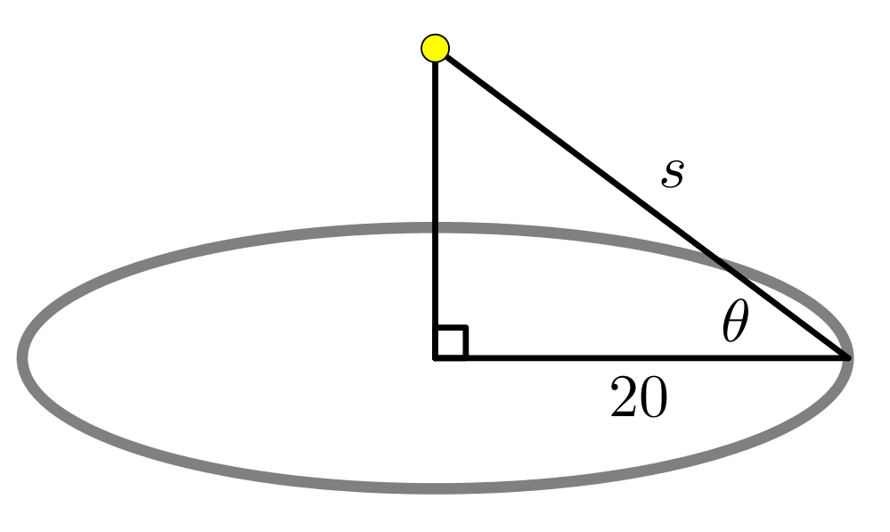
Figure 4.5.5 A solitary lampost.