8.2: The heat equation

Last updated
Save as PDF

Page ID: 35372

\( \newcommand{\vecs}[1]{\overset { \scriptstyle \rightharpoonup} {\mathbf{#1}} } \) \( \newcommand{\vecd}[1]{\overset{-\!-\!\rightharpoonup}{\vphantom{a}\smash {#1}}} \)\(\newcommand{\id}{\mathrm{id}}\) \( \newcommand{\Span}{\mathrm{span}}\) \( \newcommand{\kernel}{\mathrm{null}\,}\) \( \newcommand{\range}{\mathrm{range}\,}\) \( \newcommand{\RealPart}{\mathrm{Re}}\) \( \newcommand{\ImaginaryPart}{\mathrm{Im}}\) \( \newcommand{\Argument}{\mathrm{Arg}}\) \( \newcommand{\norm}[1]{\| #1 \|}\) \( \newcommand{\inner}[2]{\langle #1, #2 \rangle}\) \( \newcommand{\Span}{\mathrm{span}}\) \(\newcommand{\id}{\mathrm{id}}\) \( \newcommand{\Span}{\mathrm{span}}\) \( \newcommand{\kernel}{\mathrm{null}\,}\) \( \newcommand{\range}{\mathrm{range}\,}\) \( \newcommand{\RealPart}{\mathrm{Re}}\) \( \newcommand{\ImaginaryPart}{\mathrm{Im}}\) \( \newcommand{\Argument}{\mathrm{Arg}}\) \( \newcommand{\norm}[1]{\| #1 \|}\) \( \newcommand{\inner}[2]{\langle #1, #2 \rangle}\) \( \newcommand{\Span}{\mathrm{span}}\)\(\newcommand{\AA}{\unicode[.8,0]{x212B}}\)

\[\underset{\text{heat equation in two dimensions}}{u_t=c^2(u_{xx}+u_{yy})}\]

The unknown function \(u\) has three independent variables: \(t\), \(x\), and \(y\) with \(c\) is an arbitrary constant. The independent variables \(x\) and \(y\) are considered to be spatial variables, and the variable \(t\) represents time.

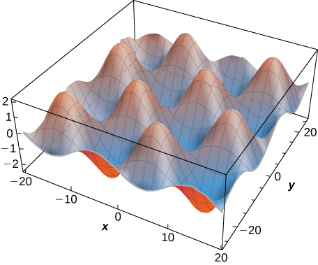
Example \(\PageIndex{1}\): A Solution to the Heat Equation

Verify that

\[u(x,y,t)=2\sin \left(\dfrac{x}{3} \right)\sin\left(\dfrac{y}{4} \right)e^{−25t/16} \nonumber\]

is a solution to the heat equation

\[u_t=9(u_{xx}+u_{yy}). \nonumber\]

Hint: Calculate the partial derivatives and substitute into the right-hand side.

Since the solution to the two-dimensional heat equation is a function of three variables, it is not easy to create a visual representation of the solution. We can graph the solution for fixed values of t, which amounts to snapshots of the heat distributions at fixed times. These snapshots show how the heat is distributed over a two-dimensional surface as time progresses. The graph of the preceding solution at time \(t=0\) appears in Figure \(\PageIndex{3}\). As time progresses, the extremes level out, approaching zero as t approaches infinity.

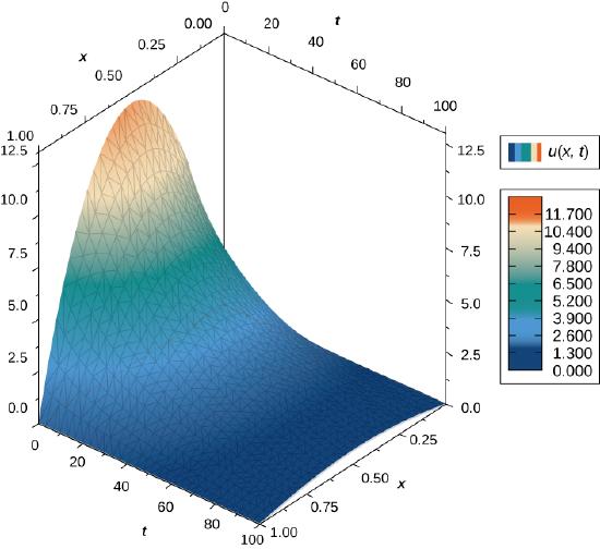
If we consider the heat equation in one dimension, then it is possible to graph the solution over time. The heat equation in one dimension becomes

\[u_t=c^2u_{xx},\]

where \(c^2\) represents the thermal diffusivity of the material in question. A solution of this differential equation can be written in the form

\[u_m(x,t)=e^{−π^2m^2c^2t}\sin(mπx)\]

where \(m\) is any positive integer. A graph of this solution using \(m=1\) appears in Figure \(\PageIndex{4}\), where the initial temperature distribution over a wire of length \(1\) is given by \(u(x,0)=\sin πx.\) Notice that as time progresses, the wire cools off. This is seen because, from left to right, the highest temperature (which occurs in the middle of the wire) decreases and changes color from red to blue.

alt — Figure \(\PageIndex{4}\): Graph of a solution of the heat equation in one dimension over time.