4.7: Exponential and Logarithmic Models

Modeling Exponential Growth and Decay

In real-world applications, we need to model the behavior of a function. In mathematical modeling, we choose a familiar general function with properties that suggest that it will model the real-world phenomenon we wish to analyze. In the case of rapid growth, we may choose the exponential growth function:

\[y=A_0e^{kt}\]

where \(A_0\) is equal to the value at time zero, \(e\) is Euler’s constant, and \(k\) is a positive constant that determines the rate (percentage) of growth. We may use the exponential growth function in applications involving doubling time, the time it takes for a quantity to double. Such phenomena as wildlife populations, financial investments, biological samples, and natural resources may exhibit growth based on a doubling time. In some applications, however, as we will see when we discuss the logistic equation, the logistic model sometimes fits the data better than the exponential model.

On the other hand, if a quantity is falling rapidly toward zero, without ever reaching zero, then we should probably choose the exponential decay model. Again, we have the form \(y=A_0e^{kt}\) where \(A_0\) is the starting value, and \(e\) is Euler’s constant. Now \(k\) is a negative constant that determines the rate of decay. We may use the exponential decay model when we are calculating half-life, or the time it takes for a substance to exponentially decay to half of its original quantity. We use half-life in applications involving radioactive isotopes.

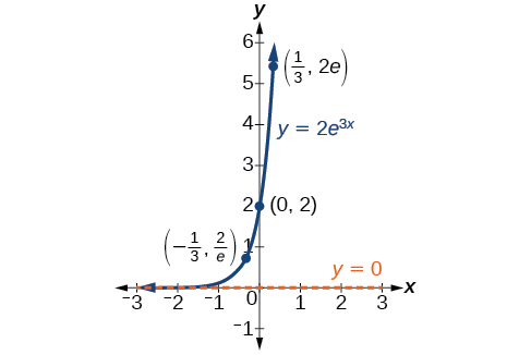
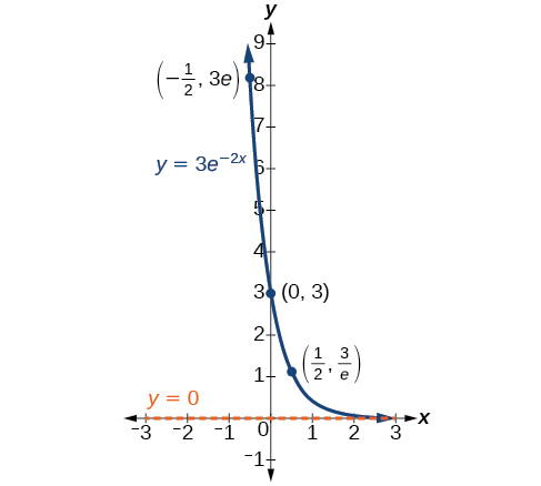
In our choice of a function to serve as a mathematical model, we often use data points gathered by careful observation and measurement to construct points on a graph and hope we can recognize the shape of the graph. Exponential growth and decay graphs have a distinctive shape, as we can see in Figure \(\PageIndex{2}\) and Figure \(\PageIndex{3}\). It is important to remember that, although parts of each of the two graphs seem to lie on the \(x\)-axis, they are really a tiny distance above the \(x\)-axis.

Figure \(\PageIndex{2}\): A graph showing exponential growth. The equation is \(y=2e^{3x}\).

Figure \(\PageIndex{3}\): A graph showing exponential decay. The equation is \(y=3e^{−2x}\).

Exponential growth and decay often involve very large or very small numbers. To describe these numbers, we often use orders of magnitude. The order of magnitude is the power of ten, when the number is expressed in scientific notation, with one digit to the left of the decimal. For example, the distance to the nearest star, Proxima Centauri, measured in kilometers, is \(40,113,497,200,000\) kilometers. Expressed in scientific notation, this is \(4.01134972 × 1013\). So, we could describe this number as having order of magnitude \(1013\).

\(y=a_0e^{kt}\)

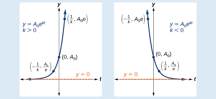
An exponential function with the form \(y=A_0e^{kt}\) has the following characteristics:

• one-to-one function
• horizontal asymptote: \(y=0\)
• domain: \((–\infty, \infty)\)
• range: \((0,\infty)\)
• \(x\) intercept: none
• \(y\)-intercept: \((0,A_0)\)
• increasing if \(k>0\) (see Figure \(\PageIndex{4}\))
• decreasing if \(k<0\) (see Figure \(\PageIndex{4}\))

Figure \(\PageIndex{4}\): An exponential function models exponential growth when \(k>0\) and exponential decay when \(k<0\).

Using Newton’s Law of Cooling

Exponential decay can also be applied to temperature. When a hot object is left in surrounding air that is at a lower temperature, the object’s temperature will decrease exponentially, leveling off as it approaches the surrounding air temperature. On a graph of the temperature function, the leveling off will correspond to a horizontal asymptote at the temperature of the surrounding air. Unless the room temperature is zero, this will correspond to a vertical shift of the generic exponential decay function. This translation leads to Newton’s Law of Cooling, the scientific formula for temperature as a function of time as an object’s temperature is equalized with the ambient temperature

\(T(t)=ae^{kt}+T_s\)

This formula is derived as follows:

\[\begin{align*} T(t)&= Ab^{ct}+T_s\\ T(t)&= Ae^{\ln(b^{ct})}+T_s \qquad \text{Laws of logarithms}\\ T(t)&= Ae^{ct\ln b}+T_s \qquad \text{Laws of logarithms}\\ T(t)&= Ae^{kt}+T_s \qquad \text{Rename the constant c } ln b \text{, calling it } k\\ \end{align*}\]

NEWTON’S LAW OF COOLING

The temperature of an object, \(T\), in surrounding air with temperature \(T_s\) will behave according to the formula

\[T(t)=Ae^{kt}+T_s\]

where

• \(t\) is time
• \(A\) is the difference between the initial temperature of the object and the surroundings
• \(k\) is a constant, the continuous rate of cooling of the object

Given a set of conditions, apply Newton’s Law of Cooling.

1. Set \(T_s\) equal to the \(y\)-coordinate of the horizontal asymptote (usually the ambient temperature).
2. Substitute the given values into the continuous growth formula \(T(t)=Ae^{kt}+T_s\) to find the parameters \(A\) and \(k\).
3. Substitute in the desired time to find the temperature or the desired temperature to find the time.

Using Logistic Growth Models

Exponential growth cannot continue forever. Exponential models, while they may be useful in the short term, tend to fall apart the longer they continue. Consider an aspiring writer who writes a single line on day one and plans to double the number of lines she writes each day for a month. By the end of the month, she must write over \(17\) billion lines, or one-half-billion pages. It is impractical, if not impossible, for anyone to write that much in such a short period of time. Eventually, an exponential model must begin to approach some limiting value, and then the growth is forced to slow. For this reason, it is often better to use a model with an upper bound instead of an exponential growth model, though the exponential growth model is still useful over a short term, before approaching the limiting value.

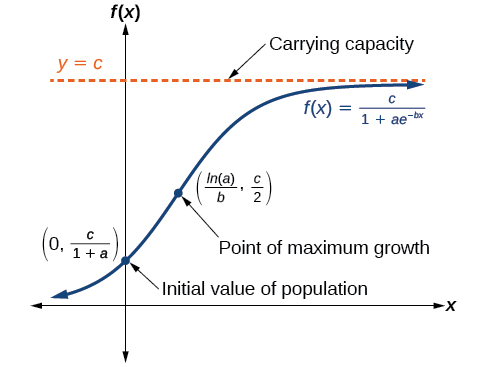
The logistic growth model is approximately exponential at first, but it has a reduced rate of growth as the output approaches the model’s upper bound, called the carrying capacity. For constants \(a\), \(b\), and \(c\), the logistic growth of a population over time \(x\) is represented by the model

\(f(x)=\dfrac{c}{1+ae^{−bx}}\)

The graph in Figure \(\PageIndex{6}\) shows how the growth rate changes over time. The graph increases from left to right, but the growth rate only increases until it reaches its point of maximum growth rate, at which point the rate of increase decreases.

Figure \(\PageIndex{6}\)

LOGISTIC GROWTH

The logistic growth model is

\[f(x)=\dfrac{c}{1+ae^{−bx}}\]

where

• \(\dfrac{c}{1+a}\) is the initial value
• \(c\) is the carrying capacity, or limiting value
• \(b\) is a constant determined by the rate of growth.

Example \(\PageIndex{6}\): Using the Logistic-Growth Model

An influenza epidemic spreads through a population rapidly, at a rate that depends on two factors: The more people who have the flu, the more rapidly it spreads, and also the more uninfected people there are, the more rapidly it spreads. These two factors make the logistic model a good one to study the spread of communicable diseases. And, clearly, there is a maximum value for the number of people infected: the entire population.

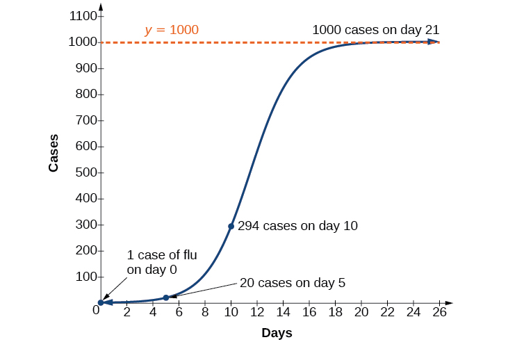
For example, at time \(t=0\) there is one person in a community of \(1,000\) people who has the flu. So, in that community, at most \(1,000\) people can have the flu. Researchers find that for this particular strain of the flu, the logistic growth constant is \(b=0.6030\). Estimate the number of people in this community who will have had this flu after ten days. Predict how many people in this community will have had this flu after a long period of time has passed.

Solution

We substitute the given data into the logistic growth model

\(f(x)=\dfrac{c}{1+ae^{−bx}}\)

Because at most \(1,000\) people, the entire population of the community, can get the flu, we know the limiting value is \(c=1000\). To find \(a\),we use the formula that the number of cases at time \(t=0\) is \(\dfrac{c}{1+a}=1\), from which it follows that \(a=999\).This model predicts that, after ten days, the number of people who have had the flu is \(f(x)=\dfrac{1000}{1+999e^{−0.6030x}}≈293.8\). Because the actual number must be a whole number (a person has either had the flu or not) we round to \(294\). In the long term, the number of people who will contract the flu is the limiting value, \(c=1000\).

Analysis

Remember that, because we are dealing with a virus, we cannot predict with certainty the number of people infected. The model only approximates the number of people infected and will not give us exact or actual values.

The graph in Figure \(\PageIndex{7}\) gives a good picture of how this model fits the data.

Figure \(\PageIndex{7}\): The graph of \(f(x)=\dfrac{1000}{1+999e^{−0.6030x}}\)

Expressing an Exponential Model in Base \(e\)

While powers and logarithms of any base can be used in modeling, the two most common bases are \(10\) and \(e\). In science and mathematics, the base \(e\) is often preferred. We can use laws of exponents and laws of logarithms to change any base to base \(e\).

Given a model with the form \(y=ab^x\), change it to the form \(y=A_0e^{kx}\).

1. Rewrite \(y=ab^x\) as \(y=ae^{\ln(b^x)}\).
2. Use the power rule of logarithms to rewrite \(y\) as \(y=ae^{x\ln(b)}=ae^{\ln{(b)}^x}\).
3. Note that \(a=A_0\) and \(k=\ln(b)\) in the equation \(y=A_0e^{kx}\).

Example \(\PageIndex{8}\): Changing to base \(e\)

Change the function \(y=2.5{(3.1)}^x\) so that this same function is written in the form \(y=A_0e^{kx}\).

Solution

The formula is derived as follows

\[\begin{align*} y&= 2.5{(3.1)}^x\\ &= 2.5e^{\ln({3.1}^x)} \qquad \text{Insert exponential and its inverse}\\ &= 2.5e^{x\ln3.1} \qquad \text{Laws of logs}\\ &= 2.5e^{(\ln3.1)x} \qquad \text{Commutative law of multiplication} \end{align*}\]