2.2: Graphs of the Secant and Cosecant Functions

Last updated
Save as PDF

Page ID: 59548

$ \newcommand{\vecs}[1]{\overset { \scriptstyle \rightharpoonup} {\mathbf{#1}} } $ $ \newcommand{\vecd}[1]{\overset{-\!-\!\rightharpoonup}{\vphantom{a}\smash {#1}}} $$\newcommand{\id}{\mathrm{id}}$ $ \newcommand{\Span}{\mathrm{span}}$ $ \newcommand{\kernel}{\mathrm{null}\,}$ $ \newcommand{\range}{\mathrm{range}\,}$ $ \newcommand{\RealPart}{\mathrm{Re}}$ $ \newcommand{\ImaginaryPart}{\mathrm{Im}}$ $ \newcommand{\Argument}{\mathrm{Arg}}$ $ \newcommand{\norm}[1]{\| #1 \|}$ $ \newcommand{\inner}[2]{\langle #1, #2 \rangle}$ $ \newcommand{\Span}{\mathrm{span}}$ $\newcommand{\id}{\mathrm{id}}$ $ \newcommand{\Span}{\mathrm{span}}$ $ \newcommand{\kernel}{\mathrm{null}\,}$ $ \newcommand{\range}{\mathrm{range}\,}$ $ \newcommand{\RealPart}{\mathrm{Re}}$ $ \newcommand{\ImaginaryPart}{\mathrm{Im}}$ $ \newcommand{\Argument}{\mathrm{Arg}}$ $ \newcommand{\norm}[1]{\| #1 \|}$ $ \newcommand{\inner}[2]{\langle #1, #2 \rangle}$ $ \newcommand{\Span}{\mathrm{span}}$$\newcommand{\AA}{\unicode[.8,0]{x212B}}$

Learning Objectives

Analyze the graphs of $y=\sec x$ and $y=\csc x$.
Graph variations of $y=\sec x$ and $y=\csc x$.

Analyzing the Graphs of $y = \sec x$ and $y = \csc x$

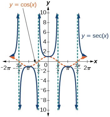
The secant function was defined by the reciprocal identity $sec \, x=\dfrac{1}{\cos x}$. Notice that the function is undefined when the cosine is $0$, leading to vertical asymptotes at $\dfrac{\pi}{2}$, $\dfrac{3\pi}{2}$ etc. Because the cosine is never more than $1$ in absolute value, the secant, being the reciprocal, will never be less than $1$ in absolute value.

We can graph $y=\sec x$ by observing the graph of the cosine function because these two functions are reciprocals of one another. See Figure $\PageIndex{1}$. The graph of the cosine is shown as a dashed orange wave so we can see the relationship. Where the graph of the cosine function decreases, the graph of the secant function increases. Where the graph of the cosine function increases, the graph of the secant function decreases. When the cosine function is zero, the secant is undefined.

The secant graph has vertical asymptotes at each value of $x$ where the cosine graph crosses the $x$-axis - this is because the inverse of 0 is undefined. We show these in the graph below with dashed vertical lines, but will not show all the asymptotes explicitly on all later graphs involving the secant and cosecant.

Note that, because cosine is an even function, secant is also an even function. That is, $\sec(−x)=\sec x$.

A graph of cosine of x and secant of x. Asymptotes for secant of x shown at -3pi/2, -pi/2, pi/2, and 3pi/2. — Figure $\PageIndex{1}$: Graph of the secant function, $f(x)=\sec x=\dfrac{1}{\cos x}$

Because there are no maximum or minimum values of a tangent function, the term amplitude cannot be interpreted as it is for the sine and cosine functions. Instead, we will use the phrase stretching/compressing factor when referring to the constant $A$.

FEATURES OF THE GRAPH OF $Y = A \sec(Bx)$

The stretching factor is $| A |$.
The period is $\dfrac{2\pi}{| B |}$.
The domain is $x≠\dfrac{\pi}{2| B |}k$, where $k$ is an odd integer.
The range is $(−∞,−|A|]∪[|A|,∞)$.
The vertical asymptotes occur at $x=\dfrac{\pi}{2| B |}k$, where $k$ is an odd integer.
There is no amplitude.
$y=A\sec(Bx)$ is an even function because cosine is an even function.

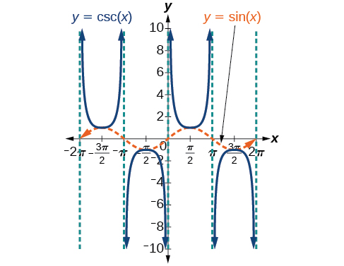
Similar to the secant, the cosecant is defined by the reciprocal identity $\csc x=\dfrac{1}{\sin x}$. Notice that the function is undefined when the sine is $0$, leading to a vertical asymptote in the graph at $0$, $\pi$, etc. Since the sine is never more than $1$ in absolute value, the cosecant, being the reciprocal, will never be less than $1$ in absolute value.

We can graph $y=\csc x$ by observing the graph of the sine function because these two functions are reciprocals of one another. See Figure $\PageIndex{2}$. The graph of sine is shown as a dashed orange wave so we can see the relationship. Where the graph of the sine function decreases, the graph of the cosecant function increases. Where the graph of the sine function increases, the graph of the cosecant function decreases.

The cosecant graph has vertical asymptotes at each value of $x$ where the sine graph crosses the $x$-axis; we show these in the graph below with dashed vertical lines.

Note that, since sine is an odd function, the cosecant function is also an odd function. That is, $\csc(−x)=−\csc x$.

The graph of cosecant, which is shown in Figure $\PageIndex{2}$, is similar to the graph of secant.

A graph of cosecant of x and sin of x. Five vertical asymptotes shown at multiples of pi. — Figure $\PageIndex{2}$: The graph of the cosecant function, $f(x)=\csc x=\frac{1}{\sin x}$

FEATURES OF THE GRAPH OF $Y = A \csc(Bx)$

The stretching factor is $| A |$.
The period is $\dfrac{2\pi}{|B|}$.
The domain is $x≠\dfrac{\pi}{|B|}k$, where $k$ is an integer.
The range is $(−∞,−|A|]∪[|A|,∞)$.
The asymptotes occur at $x=\dfrac{\pi}{| B |}k$, where $k$ is an integer.
$y=A\csc(Bx)$ is an odd function because sine is an odd function.

Graphing Variations of $y = \sec x$ and $y= \csc x$

For shifted, compressed, and/or stretched versions of the secant and cosecant functions, we locate the vertical asymptotes and also evaluate the functions for a few points (specifically the local extrema). If we want to graph only a single period, we can choose the interval for the period in more than one way. The procedure for secant is very similar, because the cofunction identity means that the secant graph is the same as the cosecant graph shifted half a period to the left. Vertical and phase shifts may be applied to the cosecant function in the same way as for the secant and other functions.The equations become the following.

\[y=A\sec(Bx−C)+D \nonumber\]

\[y=A\csc(Bx−C)+D \nonumber\]

FEATURES OF THE GRAPH OF $Y = A\sec(Bx−C)+D$

The stretching factor is $|A|$.
The period is $\dfrac{2\pi}{|B|}$.
The domain is $x≠\dfrac{C}{B}+\dfrac{\pi}{2| B |}k$,where $k$ is an odd integer.
The range is $(−∞,−|A|]∪[|A|,∞)$.
The vertical asymptotes occur at $x=\dfrac{C}{B}+\dfrac{π}{2| B |}k$,where $k$ is an odd integer.
There is no amplitude.
$y=A\sec(Bx)$ is an even function because cosine is an even function.

FEATURES OF THE GRAPH OF $Y = A\csc(Bx−C)+D$

The stretching factor is $|A|$.
The period is $\dfrac{2\pi}{|B|}$.
The domain is $x≠\dfrac{C}{B}+\dfrac{\pi}{2| B |}k$,where $k$ is an integer.
The range is $(−∞,−|A|]∪[|A|,∞)$.
The vertical asymptotes occur at $x=\dfrac{C}{B}+\dfrac{\pi}{|B|}k$,where $k$ is an integer.
There is no amplitude.
$y=A\csc(Bx)$ is an odd function because sine is an odd function.

HOWTO: Given a function of the form $y=A\sec(Bx)$, graph one period

Sketch the function $y=A\cos(Bx)$.
Draw vertical asymptotes where the curve crosses the midline, which is the $x$-axis
Fill in the secant curve in between the asymptotes. Where the cosine curve has a maximum, the secant curve will have an upward U. Where the cosine curve has a minimum, the secant curve will have a downward U.

Example $\PageIndex{1}$: Graphing a Variation of the Secant Function

Graph one period of $f(x)=2.5\sec(0.4x)$.

Solution

Step 1. Sketch a graph of the function $f(x)=2.5\cos(0.4x)$. $A=2.5$ so the stretching factor is $2.5$. $B=0.4$ so $P=\dfrac{2\pi}{0.4}=5\pi$. The period is $5\pi$ units. Dividing this by 4 gives $\dfrac{5\pi}{4}$. Each time we travel a distance of $\dfrac{5\pi}{4}$ we will be at a maximum, on the midline, or at a minimum.
Step 2. Draw vertical asymptotes where the curve crosses the midline, which is the $x$-axis
Step 3. Fill in the secant curve in between the asymptotes. Where the cosine curve has a maximum, the secant curve will have an upward U. Where the cosine curve has a minimum, the secant curve will have a downward U. Figure $\PageIndex{3}$ shows the graph. The green dashed curve is the cosine function, which acts at the "skeleton" for the secant curve. The blue dashed lines are the vertical asymptotes. The red curves are the acutal secant function.

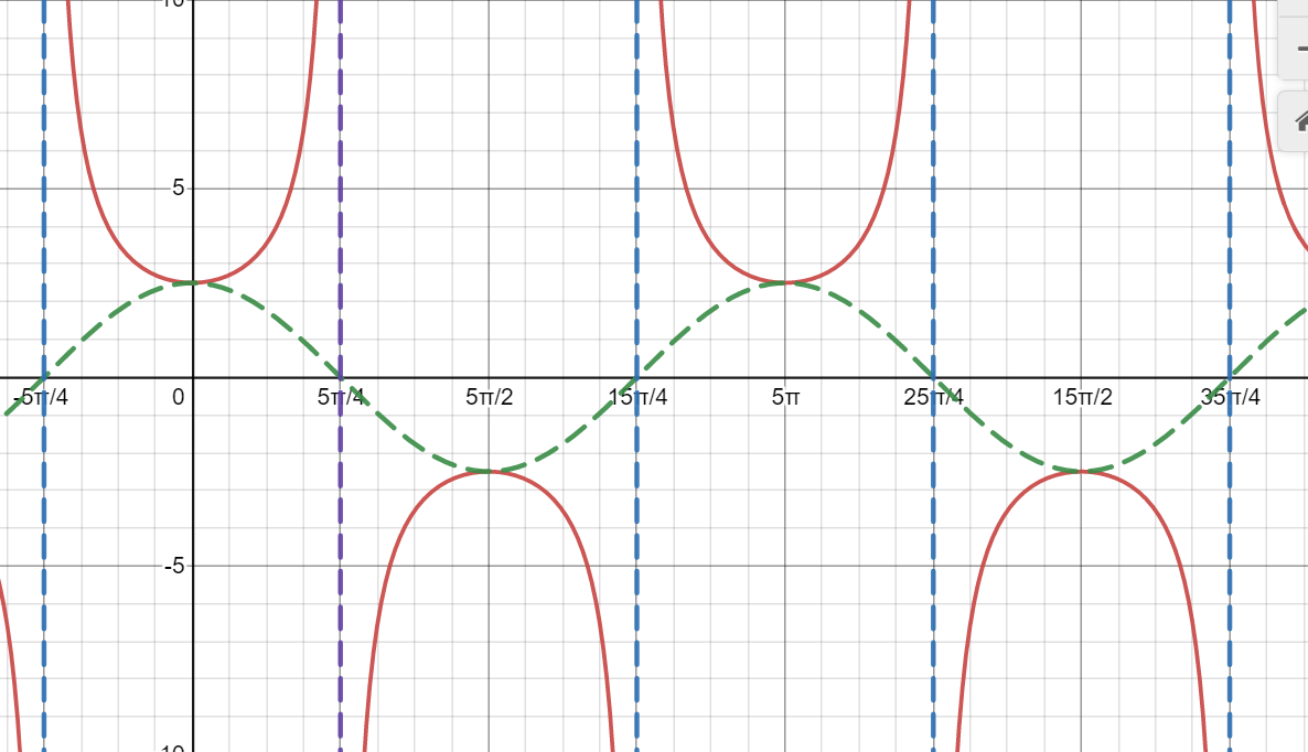
$clipboard_ee82e805893673fbf67dcaece80a3635a.png$

Figure $\PageIndex{3}$

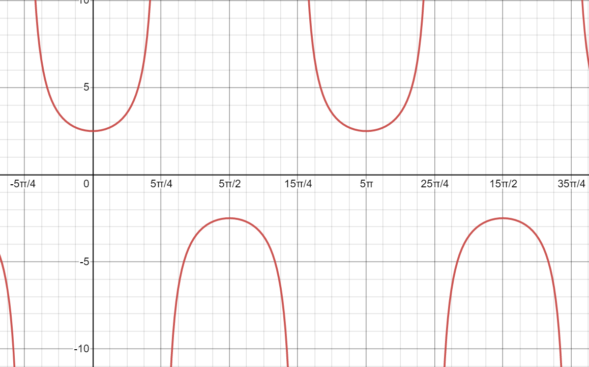
Note that in the above graph the green and blue dashed lines are not part of the secant graph, we just use them to obtain the secant graph. Only the red curves are the secant graph, as shown below.

$clipboard_e5d5e71aeda57e72590c06278771783e8.png$

Exercise $\PageIndex{1}$

Graph one period of $f(x)=−2.5\sec(0.4x)$.

Answer: This is a vertical reflection of the preceding graph because $A$ is negative.

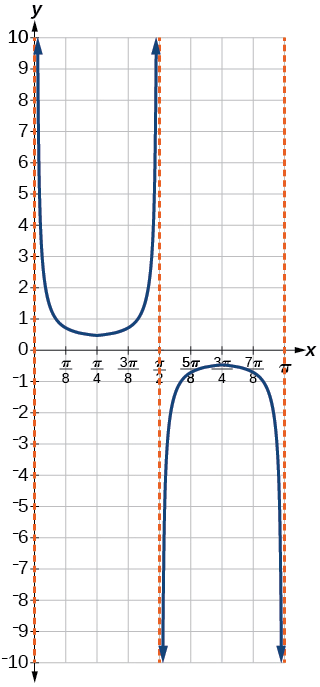
$A graph of one period of a modified secant function, which looks like an downward facing parabola and a upward facing parabola.$
Figure $\PageIndex{4}$

Q&A: Do the vertical shift and stretch/compression affect the secant’s range?

Yes. The range of $f(x)=A\sec(Bx−C)+D$ is $(−∞,−|A|+D]∪[|A|+D,∞)$.

Given a function of the form $f(x)=A\sec(Bx−C)+D$, graph one period.

Draw the graph of $f(x)=A\cos(Bx−C)+D$
Sketch the vertical asymptotes, which occur where the cosine curve passes through its midline at $y=D$
Fill in the secant curve in between the asymptotes. Where the cosine curve has a maximum, the secant curve will have an upward U. Where the cosine curve has a minimum, the secant curve will have a downward U.

Example $\PageIndex{2}$: Graphing a Variation of the Secant Function

Graph one period of $y=\sec \left (2x−\dfrac{\pi}{2} \right )+3$.

Solution

Step 1. Sketch the curve $y=\cos \left (2x−\dfrac{\pi}{2} \right )+3$.The stretching/compressing factor is $| A |=1$ so the amplitude is 1. $B=2$ so the period is $\dfrac{2\pi}{2}=\pi$. Dividing the period by 4 gives $\dfrac{\pi}{4}$. Each time we travel this distance we will be at a maximum, on the midline, or a minimum. To find the phase shift, we solve the equation $2x−\dfrac{\pi}{2}=0$, which has the solution $x=\dfrac{\pi}{4}$. There is a phase shift $\dfrac{\pi}{4}$ to the right. This means we can "start" the cosine curve at a maximum located at $\left(\dfrac{\pi}{4},4\right)$. The midline is the horizontal line $y=3$.
Step 2. Sketch the vertical asymptotes, which occur where the cosine curve passes through its midline $y=3$.
Step 3. Fill in the secant curve in between the asymptotes. Where the cosine curve has a maximum, the secant curve will have an upward U. Where the cosine curve has a minimum, the secant curve will have a downward U. Figure $\PageIndex{5}$ shows the graph. The green curve is the cosine function and the vertical blue lines are the vertical asymptotes. The curve $y=\sec \left (2x−\dfrac{\pi}{2} \right )+3$ is in red.

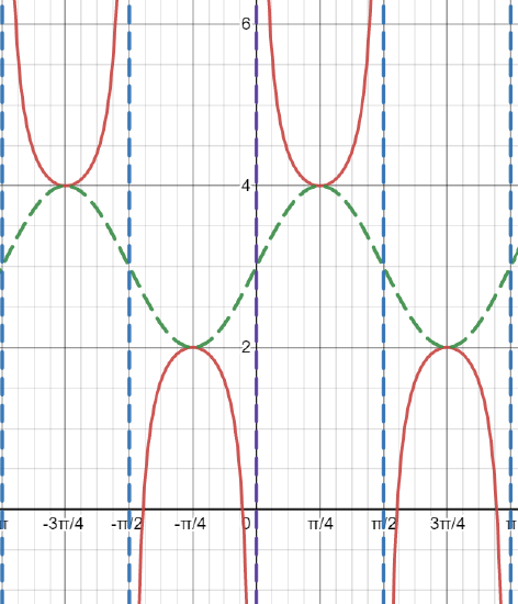
$clipboard_eee1ee4e9f705882726ae375841dbe463.png$

Figure $\PageIndex{5}$

Exercise $\PageIndex{2}$

Graph one period of $f(x)=−6\sec(4x+2)−8$.

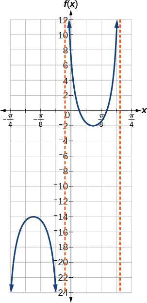
Answer: $A graph of one period of a modified secant function. There are two vertical asymptotes, one at approximately x=-pi/20 and one approximately at 3pi/16.$
Figure $\PageIndex{6}$

Q&A: The domain of $\csc \, x$ was given to be all $x$ such that $x≠k\pi$ for any integer $k$. Would the domain of $y=A\csc(Bx−C)+D$ be $x≠\dfrac{C+k\pi}{B}$?

Yes. The excluded points of the domain follow the vertical asymptotes. Their locations show the horizontal shift and compression or expansion implied by the transformation to the original function’s input.

Given a function of the form $y=A\csc(Bx)$, graph one period.

Sketch the function $y=A\sin(Bx)$.
Draw vertical asymptotes where the curve crosses the midline, which is the $x$-axis
Fill in the cosecant curve in between the asymptotes. Where the sine curve has a maximum, the cosecant curve will have an upward U. Where the sine curve has a minimum, the cosecant curve will have a downward U.

Example $\PageIndex{3}$: Graphing a Variation of the Cosecant Function

Graph one period of $f(x)=−3\csc(4x)$.

Solution

Step 1. Sketch a graph of the function $f(x)=−3\sin(4x)$. $| A |=| −3 |=3$,so the amplitude is 3. $B=4$,so $P=\dfrac{2\pi}{4}=\dfrac{\pi}{2}$. The period is $\dfrac{\pi}{2}$ units. Dividing the period by 4 gives $\dfrac{\pi}{8}$. Each time we travel a distance of $\dfrac{\pi}{8}$ the sine curve will have a maximum, be on the midline, or have a minimum. The value of $C$ is 0 so there is no phase shift, we can "start" the curve on the midline at $x=0$. The value of $D$ is 0 so there is no vertical shift - the midline is the $x$-axis.
Step 2. Draw vertical asymptotes where the curve crosses the midline, which is the $x$-axis.
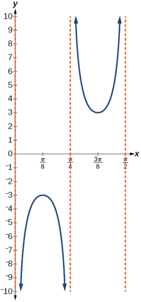
Step 3. Fill in the cosecant curve in between the asymptotes. Where the sine curve has a maximum, the cosecant curve will have an upward U. Where the sine curve has a minimum, the cosecant curve will have a downward U. Figure $\PageIndex{7}$ shows the graph over one period.

A graph of one period of a cosecant function. There are vertical asymptotes at x=0, x=pi/4, and x=pi/2. — Figure $\PageIndex{7}$

Exercise $\PageIndex{3}$

Graph $f(x)=0.5\csc(2x)$ over at least two periods.

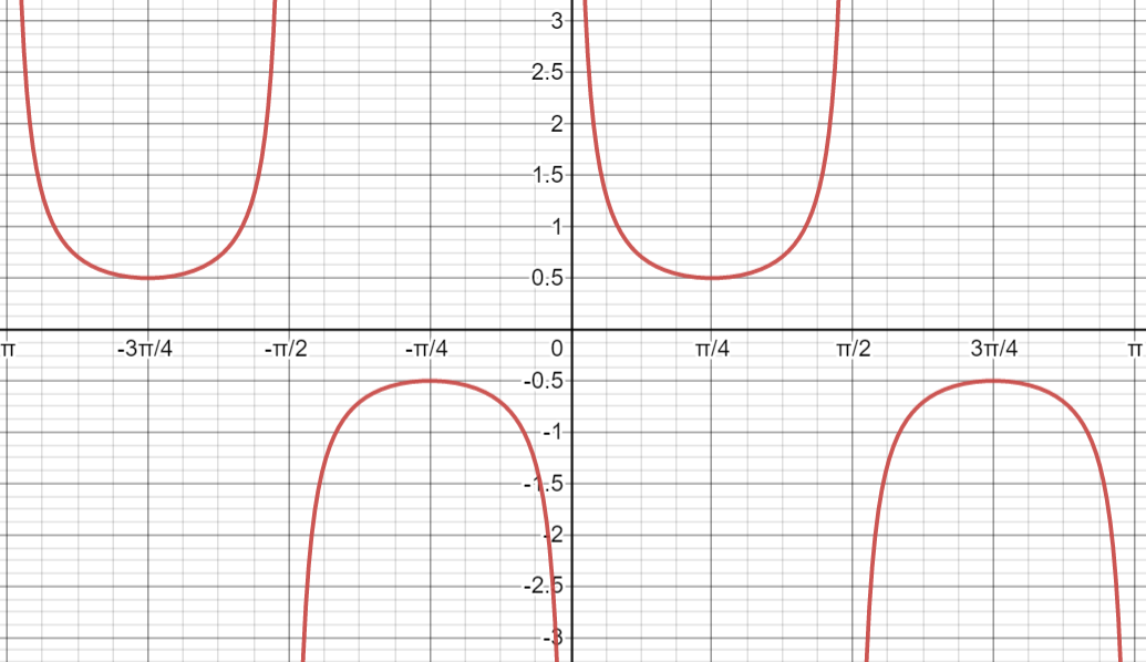
Answer: $clipboard_ef7b2e008cc3c176d99d7b5d9b50987d2.png$

Figure $\PageIndex{8}$

Given a function of the form $f(x)=A \csc(Bx−C)+D$, graph one period

Draw the graph of $f(x)=A\sin(Bx−C)+D$
Sketch the vertical asymptotes, which occur where the sine curve passes through its midline at $y=D$
Fill in the cosecant curve in between the asymptotes. Where the sine curve has a maximum, the cosecant curve will have an upward U. Where the sine curve has a minimum, the cosecant curve will have a downward U.

Example $\PageIndex{4}$: Graphing a Vertically Stretched, Horizontally Compressed, and Vertically Shifted Cosecant

Sketch a graph of $y=2\csc \left (\dfrac{\pi}{2}x \right )+1$.

Solution

Step 1. Sketch a graph of $y=2\sin \left (\dfrac{\pi}{2}x \right )+1$. $| A |=2$ so the amplitude is 2. The period is $\dfrac{2\pi}{| B |}=\dfrac{2\pi}{\dfrac{\pi}{2}}=2\pi⋅\dfrac{2}{\pi}=4$. Dividing the period by 4 gives 1. Each time we move a unit of 1 the sine curve will have a maximum, be on the midline, or have a minimum. To find the phase shift we solve the equation $\dfrac{\pi}{2}x=0$ which has a solution $x=0$. We can "start" the sine curve at $x=0$ on the midline, which is at $y=1$.
Step 2. Sketch the vertical asymptotes, which occur where the sine curve passes through its midline at $y=1$.
Step 3. Fill in the cosecant curve in between the asymptotes. Where the sine curve has a maximum, the cosecant curve will have an upward U. Where the sine curve has a minimum, the cosecant curve will have a downward U.

The graph for this function is shown in Figure $\PageIndex{9}$ in dark blue. The orange dashed line is the sine curve and the dashed vertical blue and green lines are the vertical asymptotes.

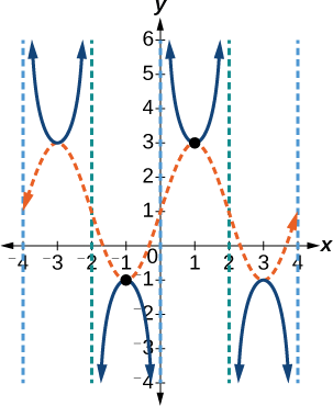
A graph of 3 periods of a modified cosecant function, with 3 vertical asymptotes, and a dotted sinusoidal function that has local maximums where the cosecant function has local minimums and local minimums where the cosecant function has local maximums. — Figure $\PageIndex{9}$: A transformed cosecant function

Analysis

The vertical asymptotes shown on the graph mark off one period of the function, and the local extrema in this interval are shown by dots. Notice how the graph of the transformed cosecant relates to the graph of $f(x)=2\sin \left (\frac{\pi}{2}x \right )+1$,shown as the orange dashed wave.

Exercise $\PageIndex{4}$

Given the graph of $f(x)=2\cos \left (\frac{\pi}{2}x \right )+1$ shown in Figure $\PageIndex{10}$, sketch the graph of $g(x)=2\sec \left (\dfrac{\pi}{2}x \right )+1$ on the same axes.

A graph of two periods of a modified cosine function. Range is [-1,3], graphed from x=-4 to x=4. — Figure $\PageIndex{10}$

Answer: $A graph of two periods of both a secant and consine function. Grpah shows that cosine function has local maximums where secant function has local minimums and vice versa.$
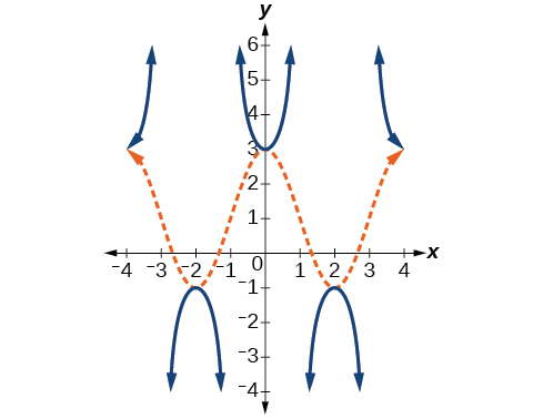
Figure $\PageIndex{18}$

Key Equations

Shifted, compressed, and/or stretched secant function	$y=A \sec(Bx−C)+D$
Shifted, compressed, and/or stretched cosecant function	$y=A \csc(Bx−C)+D$

Key Concepts

The secant and cosecant are both periodic functions with a period of $2\pi$.
$f( x )=A\sec( Bx−C )+D$ gives a shifted, compressed, and/or stretched secant function graph. See Example $\PageIndex{4}$ and Example $\PageIndex{5}$.
$f( x )=A\csc( Bx−C )+D$ gives a shifted, compressed, and/or stretched cosecant function graph. See Example $\PageIndex{6}$ and Example $\PageIndex{7}$.

Contributors and Attributions

Jay Abramson (Arizona State University) with contributing authors. Textbook content produced by OpenStax College is licensed under a Creative Commons Attribution License 4.0 license. Download for free at https://openstax.org/details/books/precalculus.

Shifted, compressed, and/or stretched secant function	\(y=A \sec(Bx−C)+D\)
Shifted, compressed, and/or stretched cosecant function	\(y=A \csc(Bx−C)+D\)

Analyzing the Graphs of \(y = \sec x\) and \(y = \csc x\)

Graphing Variations of \(y = \sec x\) and \(y= \csc x\)

Key Equations

Key Concepts

Contributors and Attributions