
4.1: Basic Inverse Trigonometric Functions
- Page ID
- 61257
\( \newcommand{\vecs}[1]{\overset { \scriptstyle \rightharpoonup} {\mathbf{#1}} } \)
\( \newcommand{\vecd}[1]{\overset{-\!-\!\rightharpoonup}{\vphantom{a}\smash {#1}}} \)
\( \newcommand{\dsum}{\displaystyle\sum\limits} \)
\( \newcommand{\dint}{\displaystyle\int\limits} \)
\( \newcommand{\dlim}{\displaystyle\lim\limits} \)
\( \newcommand{\id}{\mathrm{id}}\) \( \newcommand{\Span}{\mathrm{span}}\)
( \newcommand{\kernel}{\mathrm{null}\,}\) \( \newcommand{\range}{\mathrm{range}\,}\)
\( \newcommand{\RealPart}{\mathrm{Re}}\) \( \newcommand{\ImaginaryPart}{\mathrm{Im}}\)
\( \newcommand{\Argument}{\mathrm{Arg}}\) \( \newcommand{\norm}[1]{\| #1 \|}\)
\( \newcommand{\inner}[2]{\langle #1, #2 \rangle}\)
\( \newcommand{\Span}{\mathrm{span}}\)
\( \newcommand{\id}{\mathrm{id}}\)
\( \newcommand{\Span}{\mathrm{span}}\)
\( \newcommand{\kernel}{\mathrm{null}\,}\)
\( \newcommand{\range}{\mathrm{range}\,}\)
\( \newcommand{\RealPart}{\mathrm{Re}}\)
\( \newcommand{\ImaginaryPart}{\mathrm{Im}}\)
\( \newcommand{\Argument}{\mathrm{Arg}}\)
\( \newcommand{\norm}[1]{\| #1 \|}\)
\( \newcommand{\inner}[2]{\langle #1, #2 \rangle}\)
\( \newcommand{\Span}{\mathrm{span}}\) \( \newcommand{\AA}{\unicode[.8,0]{x212B}}\)
\( \newcommand{\vectorA}[1]{\vec{#1}} % arrow\)
\( \newcommand{\vectorAt}[1]{\vec{\text{#1}}} % arrow\)
\( \newcommand{\vectorB}[1]{\overset { \scriptstyle \rightharpoonup} {\mathbf{#1}} } \)
\( \newcommand{\vectorC}[1]{\textbf{#1}} \)
\( \newcommand{\vectorD}[1]{\overrightarrow{#1}} \)
\( \newcommand{\vectorDt}[1]{\overrightarrow{\text{#1}}} \)
\( \newcommand{\vectE}[1]{\overset{-\!-\!\rightharpoonup}{\vphantom{a}\smash{\mathbf {#1}}}} \)
\( \newcommand{\vecs}[1]{\overset { \scriptstyle \rightharpoonup} {\mathbf{#1}} } \)
\(\newcommand{\longvect}{\overrightarrow}\)
\( \newcommand{\vecd}[1]{\overset{-\!-\!\rightharpoonup}{\vphantom{a}\smash {#1}}} \)
\(\newcommand{\avec}{\mathbf a}\) \(\newcommand{\bvec}{\mathbf b}\) \(\newcommand{\cvec}{\mathbf c}\) \(\newcommand{\dvec}{\mathbf d}\) \(\newcommand{\dtil}{\widetilde{\mathbf d}}\) \(\newcommand{\evec}{\mathbf e}\) \(\newcommand{\fvec}{\mathbf f}\) \(\newcommand{\nvec}{\mathbf n}\) \(\newcommand{\pvec}{\mathbf p}\) \(\newcommand{\qvec}{\mathbf q}\) \(\newcommand{\svec}{\mathbf s}\) \(\newcommand{\tvec}{\mathbf t}\) \(\newcommand{\uvec}{\mathbf u}\) \(\newcommand{\vvec}{\mathbf v}\) \(\newcommand{\wvec}{\mathbf w}\) \(\newcommand{\xvec}{\mathbf x}\) \(\newcommand{\yvec}{\mathbf y}\) \(\newcommand{\zvec}{\mathbf z}\) \(\newcommand{\rvec}{\mathbf r}\) \(\newcommand{\mvec}{\mathbf m}\) \(\newcommand{\zerovec}{\mathbf 0}\) \(\newcommand{\onevec}{\mathbf 1}\) \(\newcommand{\real}{\mathbb R}\) \(\newcommand{\twovec}[2]{\left[\begin{array}{r}#1 \\ #2 \end{array}\right]}\) \(\newcommand{\ctwovec}[2]{\left[\begin{array}{c}#1 \\ #2 \end{array}\right]}\) \(\newcommand{\threevec}[3]{\left[\begin{array}{r}#1 \\ #2 \\ #3 \end{array}\right]}\) \(\newcommand{\cthreevec}[3]{\left[\begin{array}{c}#1 \\ #2 \\ #3 \end{array}\right]}\) \(\newcommand{\fourvec}[4]{\left[\begin{array}{r}#1 \\ #2 \\ #3 \\ #4 \end{array}\right]}\) \(\newcommand{\cfourvec}[4]{\left[\begin{array}{c}#1 \\ #2 \\ #3 \\ #4 \end{array}\right]}\) \(\newcommand{\fivevec}[5]{\left[\begin{array}{r}#1 \\ #2 \\ #3 \\ #4 \\ #5 \\ \end{array}\right]}\) \(\newcommand{\cfivevec}[5]{\left[\begin{array}{c}#1 \\ #2 \\ #3 \\ #4 \\ #5 \\ \end{array}\right]}\) \(\newcommand{\mattwo}[4]{\left[\begin{array}{rr}#1 \amp #2 \\ #3 \amp #4 \\ \end{array}\right]}\) \(\newcommand{\laspan}[1]{\text{Span}\{#1\}}\) \(\newcommand{\bcal}{\cal B}\) \(\newcommand{\ccal}{\cal C}\) \(\newcommand{\scal}{\cal S}\) \(\newcommand{\wcal}{\cal W}\) \(\newcommand{\ecal}{\cal E}\) \(\newcommand{\coords}[2]{\left\{#1\right\}_{#2}}\) \(\newcommand{\gray}[1]{\color{gray}{#1}}\) \(\newcommand{\lgray}[1]{\color{lightgray}{#1}}\) \(\newcommand{\rank}{\operatorname{rank}}\) \(\newcommand{\row}{\text{Row}}\) \(\newcommand{\col}{\text{Col}}\) \(\renewcommand{\row}{\text{Row}}\) \(\newcommand{\nul}{\text{Nul}}\) \(\newcommand{\var}{\text{Var}}\) \(\newcommand{\corr}{\text{corr}}\) \(\newcommand{\len}[1]{\left|#1\right|}\) \(\newcommand{\bbar}{\overline{\bvec}}\) \(\newcommand{\bhat}{\widehat{\bvec}}\) \(\newcommand{\bperp}{\bvec^\perp}\) \(\newcommand{\xhat}{\widehat{\xvec}}\) \(\newcommand{\vhat}{\widehat{\vvec}}\) \(\newcommand{\uhat}{\widehat{\uvec}}\) \(\newcommand{\what}{\widehat{\wvec}}\) \(\newcommand{\Sighat}{\widehat{\Sigma}}\) \(\newcommand{\lt}{<}\) \(\newcommand{\gt}{>}\) \(\newcommand{\amp}{&}\) \(\definecolor{fillinmathshade}{gray}{0.9}\)Learning Objectives
- Understand and evaluate inverse trigonometric functions.
- Extend the inverse trigonometric functions to include the \(\csc^{-1}\), \(\sec^{-1}\), and \(\cot^{-1}\) functions.
- Apply inverse trigonometric functions to the critical values on the unit circle.
For any right triangle, given one other angle and the length of one side, we can figure out what the other angles and sides are. But what if we are given only two sides of a right triangle? We need a procedure that leads us from a ratio of sides to an angle. This is where the notion of an inverse to a trigonometric function comes into play. In this section, we will explore the inverse trigonometric functions.
Understanding and Using the Inverse Sine, Cosine, and Tangent Functions
In order to use inverse trigonometric functions, we need to understand that an inverse trigonometric function “undoes” what the original trigonometric function “does,” as is the case with any other function and its inverse. In other words, the domain of the inverse function is the range of the original function, and vice versa, as summarized in Figure \(\PageIndex{1}\).

For example, if \(f(x)=\sin\space x\), then we would write \(f^{−1}(x)={\sin}^{−1}x\). Be aware that \({\sin}^{−1}x\) does not mean \(\dfrac{1}{\sin\space x}\). The following examples illustrate the inverse trigonometric functions:
- Since \(\sin\left(\dfrac{\pi}{6}\right)=\dfrac{1}{2}\), then \(\dfrac{\pi}{6}={\sin}^{−1}\left(\dfrac{1}{2}\right)\).
- Since \(\cos(\pi)=−1\), then \(\pi={\cos}^{−1}(−1)\).
- Since \(\tan\left (\dfrac{\pi}{4}\right )=1\), then \(\dfrac{\pi}{4}={\tan}^{−1}(1)\).
In previous sections, we evaluated the trigonometric functions at various angles, but at times we need to know what angle would yield a specific sine, cosine, or tangent value. For this, we need inverse functions. Recall that, for a one-to-one function, if \(f(a)=b\), then an inverse function would satisfy \(f^{−1}(b)=a\).
Bear in mind that the sine, cosine, and tangent functions are not one-to-one functions. The graph of each function would fail the horizontal line test. In fact, no periodic function can be one-to-one because each output in its range corresponds to at least one input in every period, and there are an infinite number of periods. As with other functions that are not one-to-one, we will need to restrict the domain of each function to yield a new function that is one-to-one. We choose a domain for each function that includes the number 0. Figure \(\PageIndex{2}\) shows the graph of the sine function limited to \(\left[ −\dfrac{\pi}{2},\dfrac{\pi}{2} \right]\) and the graph of the cosine function limited to \([ 0,\pi ]\).
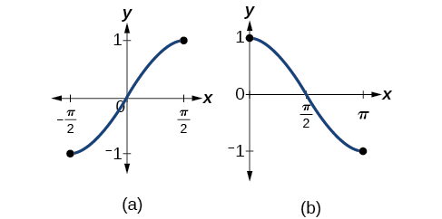
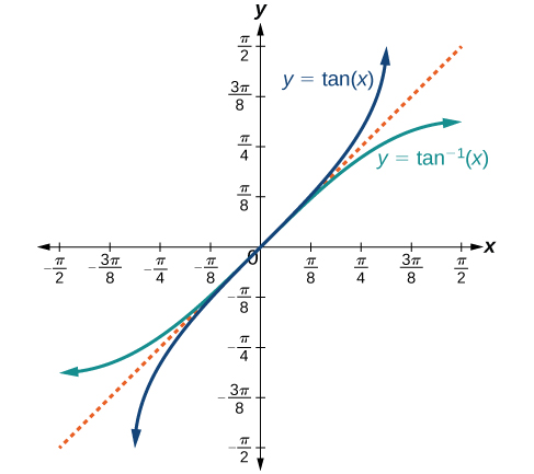
Figure \(\PageIndex{3}\) shows the graph of the tangent function limited to \(\left(−\dfrac{\pi}{2},\dfrac{\pi}{2}\right)\).
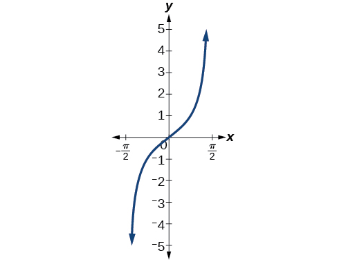
These conventional choices for the restricted domain are somewhat arbitrary, but they have important, helpful characteristics. Each domain includes the origin and some positive values, and most importantly, each results in a one-to-one function that is invertible. The conventional choice for the restricted domain of the tangent function also has the useful property that it extends from one vertical asymptote to the next instead of being divided into two parts by an asymptote.
On these restricted domains, we can define the inverse trigonometric functions.
- The inverse sine function \(y={\sin}^{−1}x\) means \(x=\sin\space y\). The inverse sine function is sometimes called the arcsine function, and notated \(\arcsin\space x\).
\(y={\sin}^{−1}x\) has domain \([−1,1]\) and range \(\left[−\frac{\pi}{2},\frac{\pi}{2}\right]\)
- The inverse cosine function \(y={\cos}^{−1}x\) means \(x=\cos\space y\). The inverse cosine function is sometimes called the arccosine function, and notated \(\arccos\space x\).
\(y={\cos}^{−1}x\) has domain \([−1,1]\) and range \([0,π]\)
- The inverse tangent function \(y={\tan}^{−1}x\) means \(x=\tan\space y\). The inverse tangent function is sometimes called the arctangent function, and notated \(\arctan\space x\).
\(y={\tan}^{−1}x\) has domain \((−\infty,\infty)\) and range \(\left(−\frac{\pi}{2},\frac{\pi}{2}\right)\)
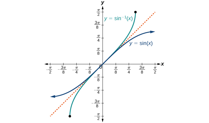
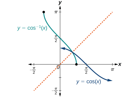
The graphs of the inverse functions are shown in Figures \(\PageIndex{4}\) - \(\PageIndex{6}\). Notice that the output of each of these inverse functions is a number, an angle in radian measure. We see that \({\sin}^{−1}x\) has domain \([ −1,1 ]\) and range \(\left[ −\dfrac{\pi}{2},\dfrac{\pi}{2} \right]\), \({\cos}^{−1}x\) has domain \([ −1,1 ]\) and range \([0,\pi]\), and \({\tan}^{−1}x\) has domain of all real numbers and range \(\left(−\dfrac{\pi}{2},\dfrac{\pi}{2}\right)\). To find the domain and range of inverse trigonometric functions, switch the domain and range of the original functions. Each graph of the inverse trigonometric function is a reflection of the graph of the original function about the line \(y=x\).
RELATIONS FOR INVERSE SINE, COSINE, AND TANGENT FUNCTIONS
For angles in the interval \(\left[ −\dfrac{\pi}{2},\dfrac{\pi}{2} \right]\), if \(\sin y=x\), then \({\sin}^{−1}x=y\).
For angles in the interval \([ 0,\pi ]\), if \(\cos y=x\), then \({\cos}^{−1}x=y\).
For angles in the interval \(\left(−\dfrac{\pi}{2},\dfrac{\pi}{2}\right )\), if \(\tan y=x\),then \({\tan}^{−1}x=y\).
Example \(\PageIndex{1}\): Writing a Relation for an Inverse Function
Given \(\sin\left(\dfrac{5\pi}{12}\right)≈0.96593\), write a relation involving the inverse sine.
Solution
Use the relation for the inverse sine. If \(\sin y=x\), then \({\sin}^{−1}x=y\).
In this problem, \(x=0.96593\), and \(y=\dfrac{5\pi}{12}\).
\({\sin}^{−1}(0.96593)≈\dfrac{5\pi}{12}\)
Exercise \(\PageIndex{1}\)
Given \(\cos(0.5)≈0.8776\),write a relation involving the inverse cosine.
- Answer
-
\(\arccos(0.8776)≈0.5\)
Finding the Exact Value of Expressions Involving the Inverse Sine, Cosine, and Tangent Functions
Now that we can identify inverse functions, we will learn to evaluate them. For most values in their domains, we must evaluate the inverse trigonometric functions by using a calculator, interpolating from a table, or using some other numerical technique. Just as we did with the original trigonometric functions, we can give exact values for the inverse functions when we are using the special angles, specifically \(\dfrac{\pi}{6}\)(30°), \(\dfrac{\pi}{4}\)(45°), and \(\dfrac{\pi}{3}\)(60°), and their reflections into other quadrants.
Given a “special” input value, evaluate an inverse trigonometric function.
- Find angle \(x\) for which the original trigonometric function has an output equal to the given input for the inverse trigonometric function.
- If \(x\) is not in the defined range of the inverse, find another angle \(y\) that is in the defined range and has the same sine, cosine, or tangent as \(x\),depending on which corresponds to the given inverse function.
Example \(\PageIndex{2}\): Evaluating Inverse Trigonometric Functions for Special Input Values
Evaluate each of the following.
- \({\sin}^{−1}\left(\dfrac{1}{2}\right)\)
- \({\sin}^{−1}\left(−\dfrac{\sqrt{2}}{2}\right)\)
- \({\cos}^{−1}\left(−\dfrac{\sqrt{3}}{2}\right)\)
- \({\tan}^{−1}(1)\)
Solution
- Evaluating \({\sin}^{−1}\left(\dfrac{1}{2}\right)\) is the same as determining the angle that would have a sine value of \(\dfrac{1}{2}\). In other words, what angle \(x\) would satisfy \(\sin(x)=\dfrac{1}{2}\)? There are multiple values that would satisfy this relationship, such as \(\dfrac{\pi}{6}\) and \(\dfrac{5\pi}{6}\), but we know we need the angle in the interval \(\left[ −\dfrac{\pi}{2},\dfrac{\pi}{2} \right]\), so the answer will be \({\sin}^{−1}\left (\dfrac{1}{2}\right)=\dfrac{\pi}{6}\). Remember that the inverse is a function, so for each input, we will get exactly one output.
- To evaluate \({\sin}^{−1}\left(−\dfrac{\sqrt{2}}{2}\right)\), we know that \(\dfrac{5\pi}{4}\) and \(\dfrac{7\pi}{4}\) both have a sine value of \(-\dfrac{\sqrt{2}}{2}\), but neither is in the interval \(\left[ −\dfrac{\pi}{2},\dfrac{\pi}{2} \right]\). For that, we need the negative angle coterminal with \(\dfrac{7\pi}{4}\): \({\sin}^{−1}\left(−\dfrac{\sqrt{2}}{2}\right)=−\dfrac{\pi}{4}\).
- To evaluate \({\cos}^{−1}\left(−\dfrac{\sqrt{3}}{2}\right)\), we are looking for an angle in the interval \([ 0,\pi ]\) with a cosine value of \(-\dfrac{\sqrt{3}}{2}\). The angle that satisfies this is \({\cos}^{−1}\left(−\dfrac{\sqrt{3}}{2}\right)=\dfrac{5\pi}{6}\).
- Evaluating \({\tan}^{−1}(1)\), we are looking for an angle in the interval \(\left(−\dfrac{\pi}{2},\dfrac{\pi}{2}\right)\) with a tangent value of \(1\). The correct angle is \({\tan}^{−1}(1)=\dfrac{\pi}{4}\).
Exercise \(\PageIndex{2}\)
Evaluate each of the following.
- \({\sin}^{−1}(−1)\)
- \({\tan}^{−1}(−1)\)
- \({\cos}^{−1}(−1)\)
- \({\cos}^{−1}\left(\dfrac{1}{2}\right)\)
- Answer a
-
\(-\dfrac{\pi}{2}\)
- Answer b
-
\(-\dfrac{\pi}{4}\)
- Answer c
-
\(\pi\)
- Answer d
-
\(\dfrac{\pi}{3}\)
Using a Calculator to Evaluate Inverse Trigonometric Functions
To evaluate inverse trigonometric functions that do not involve the special angles discussed previously, we will need to use a calculator or other type of technology. Most scientific calculators and calculator-emulating applications have specific keys or buttons for the inverse sine, cosine, and tangent functions. These may be labeled, for example, SIN-1, ARCSIN, or ASIN.
In the previous chapter, we worked with trigonometry on a right triangle to solve for the sides of a triangle given one side and an additional angle. Using the inverse trigonometric functions, we can solve for the angles of a right triangle given two sides, and we can use a calculator to find the values to several decimal places.
In these examples and exercises, the answers will be interpreted as angles and we will use \(\theta\) as the independent variable. The value displayed on the calculator may be in degrees or radians, so be sure to set the mode appropriate to the application.
Example \(\PageIndex{3}\): Evaluating the Inverse Sine on a Calculator
Evaluate \({\sin}^{−1}(0.97)\) using a calculator.
Solution
Because the output of the inverse function is an angle, the calculator will give us a degree value if in degree mode and a radian value if in radian mode. Calculators also use the same domain restrictions on the angles as we are using.
In radian mode, \({\sin}^{−1}(0.97)≈1.3252\). In degree mode, \({\sin}^{−1}(0.97)≈75.93°\). Note that in calculus and beyond we will use radians in almost all cases.
Exercise \(\PageIndex{3}\)
Evaluate \({\cos}^{−1}(−0.4)\) using a calculator.
- Answer
-
\(1.9823\) or \(113.578^{\circ}\)
Given two sides of a right triangle like the one shown in Figure 8.4.7, find an angle.
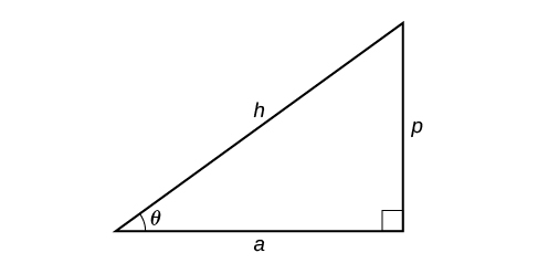
- If one given side is the hypotenuse of length \(h\) and the side of length \(a\) adjacent to the desired angle is given, use the equation \(\theta={\cos}^{−1}\left(\dfrac{a}{h}\right)\).
- If one given side is the hypotenuse of length \(h\) and the side of length \(p\) opposite to the desired angle is given, use the equation \(\theta={\sin}^{−1}\left(\dfrac{p}{h}\right)\).
- If the two legs (the sides adjacent to the right angle) are given, then use the equation \(\theta={\tan}^{−1}\left(\dfrac{p}{a}\right)\).
Example \(\PageIndex{4}\): Applying the Inverse Cosine to a Right Triangle
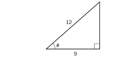
Solve the triangle in Figure \(\PageIndex{8}\) for the angle \(\theta\).
Solution
Because we know the hypotenuse and the side adjacent to the angle, it makes sense for us to use the cosine function.
\[\begin{align*} \cos \theta&= \dfrac{9}{12}\\ \theta&= {\cos}^{-1}\left(\dfrac{9}{12}\right)\qquad \text{Apply definition of the inverse}\\ \theta&\approx 0.7227\qquad \text{or about } 41.4096^{\circ} \text{ Evaluate} \end{align*}\]
Exercise \(\PageIndex{4}\)
Solve the triangle in Figure \(\PageIndex{9}\) for the angle \(\theta\).

- Answer
-
\({\sin}^{−1}(0.6)=36.87°=0.6435\) radians
Finding Exact Values of Composite Functions with Inverse Trigonometric Functions
There are times when we need to compose a trigonometric function with an inverse trigonometric function. In these cases, we can usually find exact values for the resulting expressions without resorting to a calculator. Even when the input to the composite function is a variable or an expression, we can often find an expression for the output. To help sort out different cases, let \(f(x)\) and \(g(x)\) be two different trigonometric functions belonging to the set{ \(\sin(x)\),\(\cos(x)\),\(\tan(x)\) } and let \(f^{-1}(y)\) and \(g^{-1}(y)\) be their inverses.
Evaluating Compositions of the Form \(f(f^{-1}(y))\) and \(f^{-1}(f(x))\)
For any trigonometric function,\(f(f^{-1}(y))=y\) for all \(y\) in the proper domain for the given function. This follows from the definition of the inverse and from the fact that the range of \(f\) was defined to be identical to the domain of \(f^{−1}\). However, we have to be a little more careful with expressions of the form \(f^{-1}(f(x))\).
COMPOSITIONS OF A TRIGONOMETRIC FUNCTION AND ITS INVERSE
\[\begin{align*} \sin({\sin}^{-1}x)&= x\qquad \text{for } -1\leq x\leq 1\\ \cos({\cos}^{-1}x)&= x\qquad \text{for } -1\leq x\leq 1\\ \tan({\tan}^{-1}x)&= x\qquad \text{for } -\infty<x<\infty\\ {\sin}^{-1}(\sin x)&= x\qquad \text{only for } -\dfrac{\pi}{2}\leq x\leq \dfrac{\pi}{2}\\ {\cos}^{-1}(\cos x)&= x\qquad \text{only for } 0\leq x\leq \pi\\ {\tan}^{-1}(\tan x)& =x\qquad \text{only for } -\dfrac{\pi}{2}< x< \dfrac{\pi}{2} \end{align*}\]
Q&A
Is it correct that \({\sin}^{−1}(\sin x)=x\)?
No. This equation is correct ifx x belongs to the restricted domain\(\left[−\dfrac{\pi}{2},\dfrac{\pi}{2}\right]\), but sine is defined for all real input values, and for \(x\) outside the restricted interval, the equation is not correct because its inverse always returns a value in \(\left[ −\dfrac{\pi}{2},\dfrac{\pi}{2} \right]\). The situation is similar for cosine and tangent and their inverses. For example, \({\sin}^{−1}\left(\sin\left(\dfrac{3\pi}{4}\right)\right)=\dfrac{\pi}{4}\).
Given an expression of the form \(f^{-1}(f(\theta))\) where \(f(\theta)=\sin \theta\), \(\cos \theta\), or \(\tan \theta\), evaluate.
- If \(\theta\) is in the restricted domain of \(f\), then \(f^{−1}(f(\theta))=\theta\).
- If not, then find an angle \(\phi\) within the restricted domain off f such that \(f(\phi)=f(\theta)\). Then \(f^{−1}(f(\theta))=\phi\).
Example \(\PageIndex{5}\): Using Inverse Trigonometric Functions
Evaluate the following:
- \({\sin}^{−1}\left (\sin \left(\dfrac{\pi}{3}\right )\right )\)
- \({\sin}^{−1}\left (\sin \left(\dfrac{2\pi}{3}\right )\right )\)
- \({\cos}^{−1}\left (\cos \left (\dfrac{2\pi}{3}\right )\right )\)
- \({\cos}^{−1}\left (\cos \left (−\dfrac{\pi}{3}\right )\right )\)
Solution
- \(\dfrac{\pi}{3}\) is in \(\left[−\dfrac{\pi}{2},\dfrac{\pi}{2}\right]\), so \({\sin}^{−1}\left(\sin\left(\dfrac{\pi}{3}\right)\right)=\dfrac{\pi}{3}\).
- \(\dfrac{2\pi}{3}\) is not in \(\left[−\dfrac{\pi}{2},\dfrac{\pi}{2}\right]\), but \(sin\left(\dfrac{2\pi}{3}\right)=sin\left(\dfrac{\pi}{3}\right)\), so \({\sin}^{−1}\left(\sin\left(\dfrac{2\pi}{3}\right)\right)=\dfrac{\pi}{3}\).
- \(\dfrac{2\pi}{3}\) is in \([ 0,\pi ]\), so \({\cos}^{−1}\left(\cos\left(\dfrac{2\pi}{3}\right)\right)=\dfrac{2\pi}{3}\).
- \(-\dfrac{\pi}{3}\) is not in \([ 0,\pi ]\), but \(\cos\left(−\dfrac{\pi}{3}\right)=\cos\left(\dfrac{\pi}{3}\right)\) because cosine is an even function. \(\dfrac{\pi}{3}\) is in \([ 0,\pi ]\), so \({\cos}^{−1}\left(\cos\left(−\dfrac{\pi}{3}\right)\right)=\dfrac{\pi}{3}\).
Exercise \(\PageIndex{5}\)
Evaluate \({\tan}^{−1}\left(\tan\left(\dfrac{\pi}{8}\right)\right)\) and \({\tan}^{−1}\left(\tan\left(\dfrac{11\pi}{9}\right)\right)\).
- Answer
-
\(\dfrac{\pi}{8}\); \(\dfrac{2\pi}{9}\)
Key Concepts
- An inverse function is one that “undoes” another function. The domain of an inverse function is the range of the original function and the range of an inverse function is the domain of the original function.
- Because the trigonometric functions are not one-to-one on their natural domains, inverse trigonometric functions are defined for restricted domains.
- For any trigonometric function \(f(x)\), if \(x=f^{−1}(y)\), then \(f(x)=y\). However, \(f(x)=y\) only implies \(x=f^{−1}(y)\) if \(x\) is in the restricted domain of \(f\). See Example \(\PageIndex{1}\).
- Special angles are the outputs of inverse trigonometric functions for special input values; for example, \(\frac{\pi}{4}={\tan}^{−1}(1)\) and \(\frac{\pi}{6}={\sin}^{−1}(\frac{1}{2})\).See Example \(\PageIndex{2}\).
- A calculator will return an angle within the restricted domain of the original trigonometric function. See Example \(\PageIndex{3}\).
- Inverse functions allow us to find an angle when given two sides of a right triangle. See Example \(\PageIndex{4}\).
Contributors and Attributions
Jay Abramson (Arizona State University) with contributing authors. Textbook content produced by OpenStax College is licensed under a Creative Commons Attribution License 4.0 license. Download for free at https://openstax.org/details/books/precalculus.