1.3E: Exercises for Section 1.3

Last updated
Save as PDF

Page ID: 110565

$ \newcommand{\vecs}[1]{\overset { \scriptstyle \rightharpoonup} {\mathbf{#1}} } $

$ \newcommand{\vecd}[1]{\overset{-\!-\!\rightharpoonup}{\vphantom{a}\smash {#1}}} $

$ \newcommand{\id}{\mathrm{id}}$ $ \newcommand{\Span}{\mathrm{span}}$

( \newcommand{\kernel}{\mathrm{null}\,}\) $ \newcommand{\range}{\mathrm{range}\,}$

$ \newcommand{\RealPart}{\mathrm{Re}}$ $ \newcommand{\ImaginaryPart}{\mathrm{Im}}$

$ \newcommand{\Argument}{\mathrm{Arg}}$ $ \newcommand{\norm}[1]{\| #1 \|}$

$ \newcommand{\inner}[2]{\langle #1, #2 \rangle}$

$ \newcommand{\Span}{\mathrm{span}}$

$ \newcommand{\id}{\mathrm{id}}$

$ \newcommand{\Span}{\mathrm{span}}$

$ \newcommand{\kernel}{\mathrm{null}\,}$

$ \newcommand{\range}{\mathrm{range}\,}$

$ \newcommand{\RealPart}{\mathrm{Re}}$

$ \newcommand{\ImaginaryPart}{\mathrm{Im}}$

$ \newcommand{\Argument}{\mathrm{Arg}}$

$ \newcommand{\norm}[1]{\| #1 \|}$

$ \newcommand{\inner}[2]{\langle #1, #2 \rangle}$

$ \newcommand{\Span}{\mathrm{span}}$ $ \newcommand{\AA}{\unicode[.8,0]{x212B}}$

$ \newcommand{\vectorA}[1]{\vec{#1}} % arrow$

$ \newcommand{\vectorAt}[1]{\vec{\text{#1}}} % arrow$

$ \newcommand{\vectorB}[1]{\overset { \scriptstyle \rightharpoonup} {\mathbf{#1}} } $

$ \newcommand{\vectorC}[1]{\textbf{#1}} $

$ \newcommand{\vectorD}[1]{\overrightarrow{#1}} $

$ \newcommand{\vectorDt}[1]{\overrightarrow{\text{#1}}} $

$ \newcommand{\vectE}[1]{\overset{-\!-\!\rightharpoonup}{\vphantom{a}\smash{\mathbf {#1}}}} $

$ \newcommand{\vecs}[1]{\overset { \scriptstyle \rightharpoonup} {\mathbf{#1}} } $

$ \newcommand{\vecd}[1]{\overset{-\!-\!\rightharpoonup}{\vphantom{a}\smash {#1}}} $

$\newcommand{\avec}{\mathbf a}$ $\newcommand{\bvec}{\mathbf b}$ $\newcommand{\cvec}{\mathbf c}$ $\newcommand{\dvec}{\mathbf d}$ $\newcommand{\dtil}{\widetilde{\mathbf d}}$ $\newcommand{\evec}{\mathbf e}$ $\newcommand{\fvec}{\mathbf f}$ $\newcommand{\nvec}{\mathbf n}$ $\newcommand{\pvec}{\mathbf p}$ $\newcommand{\qvec}{\mathbf q}$ $\newcommand{\svec}{\mathbf s}$ $\newcommand{\tvec}{\mathbf t}$ $\newcommand{\uvec}{\mathbf u}$ $\newcommand{\vvec}{\mathbf v}$ $\newcommand{\wvec}{\mathbf w}$ $\newcommand{\xvec}{\mathbf x}$ $\newcommand{\yvec}{\mathbf y}$ $\newcommand{\zvec}{\mathbf z}$ $\newcommand{\rvec}{\mathbf r}$ $\newcommand{\mvec}{\mathbf m}$ $\newcommand{\zerovec}{\mathbf 0}$ $\newcommand{\onevec}{\mathbf 1}$ $\newcommand{\real}{\mathbb R}$ $\newcommand{\twovec}[2]{\left[\begin{array}{r}#1 \\ #2 \end{array}\right]}$ $\newcommand{\ctwovec}[2]{\left[\begin{array}{c}#1 \\ #2 \end{array}\right]}$ $\newcommand{\threevec}[3]{\left[\begin{array}{r}#1 \\ #2 \\ #3 \end{array}\right]}$ $\newcommand{\cthreevec}[3]{\left[\begin{array}{c}#1 \\ #2 \\ #3 \end{array}\right]}$ $\newcommand{\fourvec}[4]{\left[\begin{array}{r}#1 \\ #2 \\ #3 \\ #4 \end{array}\right]}$ $\newcommand{\cfourvec}[4]{\left[\begin{array}{c}#1 \\ #2 \\ #3 \\ #4 \end{array}\right]}$ $\newcommand{\fivevec}[5]{\left[\begin{array}{r}#1 \\ #2 \\ #3 \\ #4 \\ #5 \\ \end{array}\right]}$ $\newcommand{\cfivevec}[5]{\left[\begin{array}{c}#1 \\ #2 \\ #3 \\ #4 \\ #5 \\ \end{array}\right]}$ $\newcommand{\mattwo}[4]{\left[\begin{array}{rr}#1 \amp #2 \\ #3 \amp #4 \\ \end{array}\right]}$ $\newcommand{\laspan}[1]{\text{Span}\{#1\}}$ $\newcommand{\bcal}{\cal B}$ $\newcommand{\ccal}{\cal C}$ $\newcommand{\scal}{\cal S}$ $\newcommand{\wcal}{\cal W}$ $\newcommand{\ecal}{\cal E}$ $\newcommand{\coords}[2]{\left\{#1\right\}_{#2}}$ $\newcommand{\gray}[1]{\color{gray}{#1}}$ $\newcommand{\lgray}[1]{\color{lightgray}{#1}}$ $\newcommand{\rank}{\operatorname{rank}}$ $\newcommand{\row}{\text{Row}}$ $\newcommand{\col}{\text{Col}}$ $\renewcommand{\row}{\text{Row}}$ $\newcommand{\nul}{\text{Nul}}$ $\newcommand{\var}{\text{Var}}$ $\newcommand{\corr}{\text{corr}}$ $\newcommand{\len}[1]{\left|#1\right|}$ $\newcommand{\bbar}{\overline{\bvec}}$ $\newcommand{\bhat}{\widehat{\bvec}}$ $\newcommand{\bperp}{\bvec^\perp}$ $\newcommand{\xhat}{\widehat{\xvec}}$ $\newcommand{\vhat}{\widehat{\vvec}}$ $\newcommand{\uhat}{\widehat{\uvec}}$ $\newcommand{\what}{\widehat{\wvec}}$ $\newcommand{\Sighat}{\widehat{\Sigma}}$ $\newcommand{\lt}{<}$ $\newcommand{\gt}{>}$ $\newcommand{\amp}{&}$ $\definecolor{fillinmathshade}{gray}{0.9}$

For exercises 1 - 6, find the volume generated when the region between the two curves is rotated around the given axis. Use both the shell method and the washer method. Use technology to graph the functions and draw a typical slice by hand.

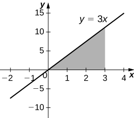
1) [T] Over the curve of $ y=3x,$ $x=0,$ and $ y=3$ rotated around the $y$-axis.

2) [T] Under the curve of $ y=3x,$ $x=0$, and $ x=3$ rotated around the $y$-axis.

Answer

$This figure is a graph in the first quadrant. It is the line y=3x. Under the line and above the x-axis there is a shaded region. The region is bounded to the right at x=3.$

$V = 54π$ units³

3) [T] Over the curve of $ y=3x,$ $x=0$, and $ y=3$ rotated around the $x$-axis.

4) [T] Under the curve of $ y=3x,$ $x=0,$ and $ x=3$ rotated around the $x$-axis.

Answer

$This figure is a graph in the first quadrant. It is the line y=3x. Under the line and above the x-axis there is a shaded region. The region is bounded to the right at x=3.$

$V = 81π$ units³

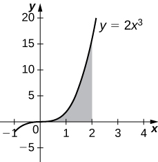
5) [T] Under the curve of $ y=2x^3,\;x=0,$ and $ x=2$ rotated around the $y$-axis.

6) [T] Under the curve of $ y=2x^3,\;x=0,$ and $ x=2$ rotated around the $x$-axis.

Answer

$This figure is a graph in the first quadrant. It is the increasing curve y=2x^3. Under the curve and above the x-axis there is a shaded region. The region is bounded to the right at x=2.$

$V = \frac{512π}{7}$ units³

For exercises 7 - 16, use shells to find the volumes of the given solids. Note that the rotated regions lie between the curve and the $x$-axis and are rotated around the $y$-axis.

7) $ y=1−x^2,$ $x=0,$ and $ x=1$

8) $ y=5x^3,$ $x=0$, and $ x=1$

Answer: $V = 2π$ units³

9) $ y=\dfrac{1}{x},$ $x=1,$ and $ x=100$

10) $ y=\sqrt{1−x^2},$ $x=0$, and $ x=1$

Answer: $V= \frac{2π}{3}$ units³

11) $ y=\dfrac{1}{1+x^2},$ $x=0$,and $ x=3$

12) $ y=\sin x^2,x=0$, and $ x=\sqrt{π}$

Answer: $V= 2π$ units³

13) $ y=\dfrac{1}{\sqrt{1−x^2}},$ $x=0$, and $ x=\frac{1}{2}$

14) $ y=\sqrt{x},$ $x=0$, and $ x=1$

Answer: $V = \frac{4π}{5}$ units³

15) $ y=(1+x^2)^3,$ $x=0$, and $ x=1$

16) $ y=5x^3−2x^4,$ $x=0$, and $ x=2$

Answer: $V= \frac{64π}{3}$ units³

For exercises 17 - 21, use shells to find the volume generated by rotating the regions between the given curve and $ y=0$ around the $x$-axis.

17) $ y=\sqrt{1−x^2},$ $x=0$, and $ x=1$

18) $ y=x^2,$ $x=0$, and $ x=2$

Answer: $V = \frac{32π}{5}$ units³

19) $ x=\dfrac{1}{1+y^2},$ $y=1$, and $ y=4$

20) $ x=\dfrac{1+y^2}{y},$ $y=0$, and $ y=2$

Answer: $V= \frac{28π}{3}$ units³

21) $ x=y^3−4y^2,$ $x=−1$, and $ x=2$

Answer: $V= \frac{84π}{5}$ units³

For exercises 22 - 26, set up integrals to use shells to find the volume generated by rotating the regions between the given curve and $ y=0$ around the $x$-axis. Use a symbolic calculator or similar technology to evaluate the integrals.

22) [T] $ y=e^x,$ $x=0$, and $ x=1$

23) [T] $ y=\ln(x),$ $x=1$, and $ x=e$

Answer: $V= π(e−2)$ units³

24) [T] $ x=\cos y,$ $y=0$, and $ y=π$

25) [T] $ x=ye^y,$ $x=−1$, and $ x=2$

26) [T] $ x=e^y\cos y,$ $x=0$, and $ x=π$

Answer: $V = e^ππ^2$ units³

For exercises 27 - 36, find the volume generated when the region between the curves is rotated around the given axis.

27) $ y=3−x$, $y=0$, $x=0$, and $ x=2$ rotated around the $y$-axis.

28) $ y=x^3$, $y=0$, $x=0$, and $ y=8$ rotated around the $y$-axis.

Answer: $ V=\frac{64π}{5}$ units³

29) $ y=x^2,$ $y=x,$ rotated around the $y$-axis.

30) $ y=\sqrt{x},$ $x=0$, and $ x=1$ rotated around the line $ x=2.$

Answer: $V=\frac{28π}{15}$ units³

31) $ y=\dfrac{1}{4−x},$ $x=1,$ and $ x=2$ rotated around the line $ x=4$.

32) $ y=\sqrt{x}$ and $ y=x^2$ rotated around the $y$-axis.

Answer: $V=\frac{3π}{10}$ units³

33) $ y=\sqrt{x}$ and $ y=x^2$ rotated around the line $ x=2$.

34) $ x=y^3,$ $y=\dfrac{1}{x},$ $x=1$, and $ y=2$ rotated around the $x$-axis.

Answer: $ \frac{52π}{5}$ units³

35) $ x=y^2$ and $ y=x$ rotated around the line $ y=2$.

36) [T] Left of $ x=\sin(πy)$, right of $ y=x$, around the $y$-axis.

Answer: $V \approx 0.9876$ units³

For exercises 37 - 44, use technology to graph the region. Determine which method you think would be easiest to use to calculate the volume generated when the function is rotated around the specified axis. Then, use your chosen method to find the volume.

37) [T] $ y=x^2$ and $ y=4x$ rotated around the $y$-axis.

38) [T] $ y=\cos(πx),y=\sin(πx),x=\frac{1}{4}$, and $ x=\frac{5}{4}$ rotated around the $y$-axis.

Answer

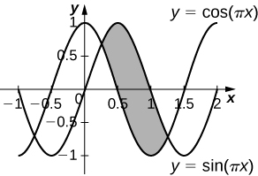
$This figure is a graph. On the graph are two curves, y=cos(pi times x) and y=sin(pi times x). They are periodic curves resembling waves. The curves intersect in the first quadrant and also the fourth quadrant. The region between the two points of intersection is shaded.$

$V = 3\sqrt{2}$ units³

39) [T] $ y=x^2−2x,\; x=2,$ and $ x=4$ rotated around the $y$-axis.

40) [T] $ y=x^2−2x,\; x=2,$ and $ x=4$ rotated around the $x$-axis.

Answer

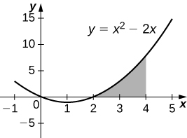
$This figure is a graph in the first quadrant. It is the parabola y=x^2-2x. . Under the curve and above the x-axis there is a shaded region. The region begins at x=2 and is bounded to the right at x=4.$

$V= \frac{496π}{15}$ units³

41) [T] $ y=3x^3−2,\; y=x$, and $ x=2$ rotated around the $x$-axis.

42) [T] $ y=3x^3−2,\; y=x$, and $ x=2$ rotated around the $y$-axis.

Answer

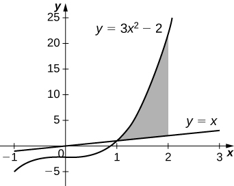
$This figure is a graph in the first quadrant. There are two curves on the graph. The first curve is y=3x^2-2 and the second curve is y=x. Between the curves there is a shaded region. The region begins at x=1 and is bounded to the right at x=2.$

$ V = \frac{398π}{15}$ units³

43) [T] $ x=\sin(πy^2)$ and $ x=\sqrt{2}y$ rotated around the $x$-axis.

44) [T] $ x=y^2,\; x=y^2−2y+1$, and $ x=2$ rotated around the $y$-axis.

Answer

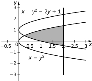
$This figure is a graph. There are two curves on the graph. The first curve is x=y^2-2y+1 and is a parabola opening to the right. The second curve is x=y^2 and is a parabola opening to the right. Between the curves there is a shaded region. The shaded region is bounded to the right at x=2.$

$ V =15.9074$ units³

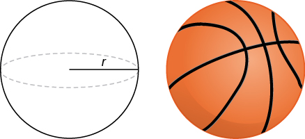
For exercises 45 - 51, use the method of shells to approximate the volumes of some common objects, which are pictured in accompanying figures.

45) Use the method of shells to find the volume of a sphere of radius $ r$.

$This figure has two images. The first is a circle with radius r. The second is a basketball.$

46) Use the method of shells to find the volume of a cone with radius $ r$ and height $ h$.

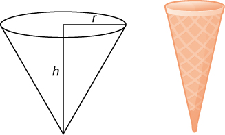
$This figure has two images. The first is an upside-down cone with radius r and height h. The second is an ice cream cone.$

Answer: $V = \frac{1}{3}πr^2h$ units³

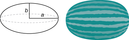
47) Use the method of shells to find the volume of an ellipse $ (x^2/a^2)+(y^2/b^2)=1$ rotated around the $x$-axis.

$This figure has two images. The first is an ellipse with a the horizontal distance from the center to the edge and b the vertical distance from the center to the top edge. The second is a watermelon.$

48) Use the method of shells to find the volume of a cylinder with radius $ r$ and height $ h$.

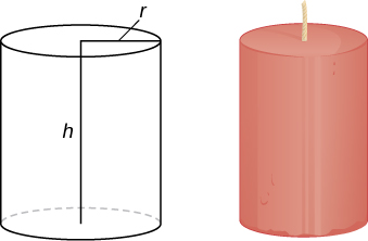
$This figure has two images. The first is a cylinder with radius r and height h. The second is a cylindrical candle.$

Answer: $V= πr^2h$ units³

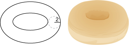
49) Use the method of shells to find the volume of the donut created when the circle $ x^2+y^2=4$ is rotated around the line $ x=4$.

$This figure has two images. The first has two ellipses, one inside of the other. The radius of the path between them is 2 units. The second is a doughnut.$

50) Consider the region enclosed by the graphs of $ y=f(x),\; y=1+f(x),\; x=0,\; y=0,$ and $ x=a>0$. What is the volume of the solid generated when this region is rotated around the $y$-axis? Assume that the function is defined over the interval $ [0,a]$.

Answer: $ V=πa^2$ units³

51) Consider the function $ y=f(x)$, which decreases from $ f(0)=b$ to $ f(1)=0$. Set up the integrals for determining the volume, using both the shell method and the disk method, of the solid generated when this region, with $ x=0$ and $ y=0$, is rotated around the $y$-axis. Prove that both methods approximate the same volume. Which method is easier to apply? (Hint: Since $ f(x)$ is one-to-one, there exists an inverse $ f^{−1}(y)$.)

Contributors

Gilbert Strang (MIT) and Edwin “Jed” Herman (Harvey Mudd) with many contributing authors. This content by OpenStax is licensed with a CC-BY-SA-NC 4.0 license. Download for free at http://cnx.org.

Search

Text Color

Text Size

Margin Size

Font Type