5.4E: Exercises for Section 5.4

In exercises 1 - 4, use appropriate substitutions to write down the Maclaurin series for the given binomial.

1) $(1−x)^{1/3}$

2) $(1+x^2)^{−1/3}$

Answer

$\displaystyle (1+x^2)^{−1/3}=\sum_{n=0}^∞\left(n^{−\frac{1}{3}}\right)x^{2n}$

3) $(1−x)^{1.01}$

4) $(1−2x)^{2/3}$

Answer

$\displaystyle (1−2x)^{2/3}=\sum_{n=0}^∞(−1)^n2^n\left(n^{\frac{2}{3}}\right)x^n$

In exercises 5 - 12, use the substitution $(b+x)^r=(b+a)^r\left(1+\dfrac{x−a}{b+a}\right)^r$ in the binomial expansion to find the Taylor series of each function with the given center.

5) $\sqrt{x+2}$ at $a=0$

6) $\sqrt{x^2+2}$ at $a=0$

Answer

$\displaystyle \sqrt{2+x^2}=\sum_{n=0}^∞2^{(1/2)−n}\left(n^{\frac{1}{2}}\right)x^{2n};(|x^2|<2)$

7) $\sqrt{x+2}$ at $a=1$

8) $\sqrt{2x−x^2}$ at $a=1$ (Hint: $2x−x^2=1−(x−1)^2$)

Answer

$\sqrt{2x−x^2}=\sqrt{1−(x−1)^2}$ so $\displaystyle \sqrt{2x−x^2}=\sum_{n=0}^∞(−1)^n\left(n^{\frac{1}{2}}\right)(x−1)^{2n}$

9) $(x−8)^{1/3}$ at $a=9$

10) $\sqrt{x}$ at $a=4$

Answer

$\sqrt{x}=2\sqrt{1+\frac{x−4}{4}}$ so $\displaystyle \sqrt{x}=\sum_{n=0}^∞2^{1−2n}\left(n^{\frac{1}{2}}\right)(x−4)^n$

11) $x^{1/3}$ at $a=27$

12) $\sqrt{x}$ at $x=9$

Answer

$\displaystyle \sqrt{x}=\sum_{n=0}^∞3^{1−3n}\left(n^{\frac{1}{2}}\right)(x−9)^n$

In exercises 13 - 14, use the binomial theorem to estimate each number, computing enough terms to obtain an estimate accurate to an error of at most 1/1000.

13) [T] $(15)^{1/4}$ using $(16−x)^{1/4}$

14) [T] $(1001)^{1/3}$ using $(1000+x)^{1/3}$

Answer

$\displaystyle 10(1+\frac{x}{1000})^{1/3}=\sum_{n=0}^∞10^{1−3n}(^{\frac{1}{3}}_n)x^n$. Using, for example, a fourth-degree estimate at $x=1$ gives $(1001)^{1/3}≈10\left(1+\left(1^{\frac{1}{3}}\right)10^{−3}+\left(2^{\frac{1}{3}}\right)10^{−6}+\left(3^{\frac{1}{3}}\right)10^{−9}+\left(3^{\frac{1}{3}}\right)10^{−12}\right)=10\left(1+\frac{1}{3.10^3}−\frac{1}{9.10^6}+\frac{5}{81.10^9}−\frac{10}{243.10^{12}}\right)=10.00333222...$ whereas $(1001)^{1/3}=10.00332222839093....$ Two terms would suffice for three-digit accuracy.

In exercises 15 - 18, use the binomial approximation $\sqrt{1−x}≈1−\frac{x}{2}−\frac{x^2}{8}−\frac{x^3}{16}−\frac{5x^4}{128}−\frac{7x^5}{256}$ for $|x|<1$ to approximate each number. Compare this value to the value given by a scientific calculator.

15) [T] $\frac{1}{\sqrt{2}}$ using $x=\frac{1}{2}$ in $(1−x)^{1/2}$

16) [T] $\sqrt{5}=5×\frac{1}{\sqrt{5}}$ using $x=\frac{4}{5}$ in $(1−x)^{1/2}$

Answer

The approximation is $2.3152$; the CAS value is $2.23….$

17) [T] $\sqrt{3}=\frac{3}{\sqrt{3}}$ using $x=\frac{2}{3}$ in $(1−x)^{1/2}$

18) [T] $\sqrt{6}$ using $x=\frac{5}{6}$ in $(1−x)^{1/2}$

Answer

The approximation is $2.583…$; the CAS value is $2.449….$

19) Integrate the binomial approximation of $\sqrt{1−x}$ to find an approximation of $\displaystyle ∫^x_0\sqrt{1−t}\,dt$.

20) [T] Recall that the graph of $\sqrt{1−x^2}$ is an upper semicircle of radius $1$. Integrate the binomial approximation of $\sqrt{1−x^2}$ up to order $8$ from $x=−1$ to $x=1$ to estimate $\frac{π}{2}$.

Answer

$\sqrt{1−x^2}=1−\frac{x^2}{2}−\frac{x^4}{8}−\frac{x^6}{16}−\frac{5x^8}{128}+⋯.$ Thus $\displaystyle ∫^1_{−1}\sqrt{1−x^2}\,dx=\left[x−\frac{x^3}{6}−\frac{x^5}{40}−\frac{x^7}{7⋅16}−\frac{5x^9}{9⋅128}+⋯\right]\Big|^1_{−1}≈2−\frac{1}{3}−\frac{1}{20}−\frac{1}{56}−\frac{10}{9⋅128}+error=1.590...$ whereas $\frac{π}{2}=1.570...$

In exercises 21 - 24, use the expansion $(1+x)^{1/3}=1+\frac{1}{3}x−\frac{1}{9}x^2+\frac{5}{81}x^3−\frac{10}{243}x^4+⋯$ to write the first five terms (not necessarily a quartic polynomial) of each expression.

21) $(1+4x)^{1/3};\;a=0$

22) $(1+4x)^{4/3};\;a=0$

Answer

$(1+x)^{4/3}=(1+x)(1+\frac{1}{3}x−\frac{1}{9}x^2+\frac{5}{81}x^3−\frac{10}{243}x^4+⋯)=1+\frac{4x}{3}+\frac{2x^2}{9}−\frac{4x^3}{81}+\frac{5x^4}{243}+⋯$

23) $(3+2x)^{1/3};\;a=−1$

24) $(x^2+6x+10)^{1/3};\;a=−3$

Answer

$(1+(x+3)^2)^{1/3}=1+\frac{1}{3}(x+3)^2−\frac{1}{9}(x+3)^4+\frac{5}{81}(x+3)^6−\frac{10}{243}(x+3)^8+⋯$

25) Use $(1+x)^{1/3}=1+\frac{1}{3}x−\frac{1}{9}x^2+\frac{5}{81}x^3−\frac{10}{243}x^4+⋯$ with $x=1$ to approximate $2^{1/3}$.

26) Use the approximation $(1−x)^{2/3}=1−\frac{2x}{3}−\frac{x^2}{9}−\frac{4x^3}{81}−\frac{7x^4}{243}−\frac{14x^5}{729}+⋯$ for $|x|<1$ to approximate $2^{1/3}=2.2^{−2/3}$.

Answer

Twice the approximation is $1.260…$ whereas $2^{1/3}=1.2599....$

27) Find the $25^{\text{th}}$ derivative of $f(x)=(1+x^2)^{13}$ at $x=0$.

28) Find the $99^{\text{th}}$ derivative of $f(x)=(1+x^4)^{25}$.

Answer

$f^{(99)}(0)=0$

In exercises 29 - 36, find the Maclaurin series of each function.

29) $f(x)=xe^{2x}$

30) $f(x)=2^x$

Answer

$\displaystyle \sum_{n=0}^∞\frac{(\ln(2)x)^n}{n!}$

31) $f(x)=\dfrac{\sin x}{x}$

32) $f(x)=\dfrac{\sin(\sqrt{x})}{\sqrt{x}},(x>0),$

Answer

For $\displaystyle x>0,\, \sin(\sqrt{x})=\sum_{n=0}^∞(−1)^n\frac{x^{(2n+1)/2}}{\sqrt{x}(2n+1)!}=\sum_{n=0}^∞(−1)^n\frac{x^n}{(2n+1)!}$.

33) $f(x)=\sin(x^2)$

34) $f(x)=e^{x^3}$

Answer

$\displaystyle e^{x^3}=\sum_{n=0}^∞\frac{x^{3n}}{n!}$

35) $f(x)=\cos^2x$ using the identity $\cos^2x=\frac{1}{2}+\frac{1}{2}\cos(2x)$

36) $f(x)=\sin^2x$ using the identity $\sin^2x=\frac{1}{2}−\frac{1}{2}\cos(2x)$

Answer

$\displaystyle \sin^2x=−\sum_{k=1}^∞\frac{(−1)^k2^{2k−1}x^{2k}}{(2k)!}$

In exercises 37 - 44, find the Maclaurin series of $\displaystyle F(x)=∫^x_0f(t)\,dt$ by integrating the Maclaurin series of $f$ term by term. If $f$ is not strictly defined at zero, you may substitute the value of the Maclaurin series at zero.

37) $\displaystyle F(x)=∫^x_0e^{−t^2}\,dt;\; f(t)=e^{−t^2}=\sum_{n=0}^∞(−1)^n\frac{t^{2n}}{n!}$

38) $\displaystyle F(x)=\tan^{−1}x;\; f(t)=\frac{1}{1+t^2}=\sum_{n=0}^∞(−1)^nt^{2n}$

Answer

$\displaystyle \tan^{−1}x=\sum_{k=0}^∞\frac{(−1)^kx^{2k+1}}{2k+1}$

39) $\displaystyle F(x)=\tanh^{−1}x; \; f(t)=\frac{1}{1−t^2}=\sum_{n=0}^∞t^{2n}$

40) $\displaystyle F(x)=\sin^{−1}x; \; f(t)=\frac{1}{\sqrt{1−t^2}}=\sum_{k=0}^∞\left(k^{\frac{1}{2}}\right)\frac{t^{2k}}{k!}$

Answer

$\displaystyle \sin^{−1}x=\sum_{n=0}^∞\left(n^{\frac{1}{2}}\right)\frac{x^{2n+1}}{(2n+1)n!}$

41) $\displaystyle F(x)=∫^x_0\frac{\sin t}{t}\,dt; \; f(t)=\frac{\sin t}{t}=\sum_{n=0}^∞(−1)^n\frac{t^{2n}}{(2n+1)!}$

42) $\displaystyle F(x)=∫^x_0\cos\left(\sqrt{t}\right)\,dt; \; f(t)=\sum_{n=0}^∞(−1)^n\frac{x^n}{(2n)!}$

Answer

$\displaystyle F(x)=\sum_{n=0}^∞(−1)^n\frac{x^{n+1}}{(n+1)(2n)!}$

43) $\displaystyle F(x)=∫^x_0\frac{1−\cos t}{t^2}\,dt; \; f(t)=\frac{1−\cos t}{t^2}=\sum_{n=0}^∞(−1)^n\frac{t^{2n}}{(2n+2)!}$

44) $\displaystyle F(x)=∫^x_0\frac{\ln(1+t)}{t}\,dt; \; f(t)=\sum_{n=0}^∞(−1)^n\frac{t^n}{n+1}$

Answer

$\displaystyle F(x)=\sum_{n=1}^∞(−1)^{n+1}\frac{x^n}{n^2}$

In exercises 45 - 52, compute at least the first three nonzero terms (not necessarily a quadratic polynomial) of the Maclaurin series of $f$.

45) $f(x)=\sin\left(x+\frac{π}{4}\right)=\sin x\cos\left(\frac{π}{4}\right)+\cos x\sin\left(\frac{π}{4}\right)$

46) $f(x)=\tan x$

Answer

$x+\dfrac{x^3}{3}+\dfrac{2x^5}{15}+⋯$

47) $f(x)=\ln(\cos x)$

48) $f(x)=e^x\cos x$

Answer

$1+x−\dfrac{x^3}{3}−\dfrac{x^4}{6}+⋯$

49) $f(x)=e^{\sin x}$

50) $f(x)=\sec^2x$

Answer

$1+x^2+\dfrac{2x^4}{3}+\dfrac{17x^6}{45}+⋯$

51) $f(x)=\tanh x$

52) $f(x)=\dfrac{\tan\sqrt{x}}{\sqrt{x}}$ (see expansion for $\tan x$)

Answer

Using the expansion for $\tan x$ gives $1+\dfrac{x}{3}+\dfrac{2x^2}{15}$.

In exercises 53 - 56, find the radius of convergence of the Maclaurin series of each function.

53) $\ln(1+x)$

54) $\dfrac{1}{1+x^2}$

Answer

$\displaystyle \frac{1}{1+x^2}=\sum_{n=0}^∞(−1)^nx^{2n}$ so $R=1$ by the ratio test.

55) $\tan^{−1}x$

56) $\ln(1+x^2)$

Answer

$\displaystyle \ln(1+x^2)=\sum_{n=1}^∞\frac{(−1)^{n−1}}{n}x^{2n}$ so $R=1$ by the ratio test.

57) Find the Maclaurin series of $\sinh x=\dfrac{e^x−e^{−x}}{2}$.

58) Find the Maclaurin series of $\cosh x=\dfrac{e^x+e^{−x}}{2}$.

Answer

Add series of $e^x$ and $e^{−x}$ term by term. Odd terms cancel and $\displaystyle \cosh x=\sum_{n=0}^∞\frac{x^{2n}}{(2n)!}$.

59) Differentiate term by term the Maclaurin series of $\sinh x$ and compare the result with the Maclaurin series of $\cosh x$.

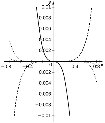
60) [T] Let $\displaystyle S_n(x)=\sum_{k=0}^n(−1)^k\frac{x^{2k+1}}{(2k+1)!}$ and $\displaystyle C_n(x)=\sum_{n=0}^n(−1)^k\frac{x^{2k}}{(2k)!}$ denote the respective Maclaurin polynomials of degree $2n+1$ of $\sin x$ and degree $2n$ of $\cos x$. Plot the errors $\dfrac{S_n(x)}{C_n(x)}−\tan x$ for $n=1,..,5$ and compare them to $x+\dfrac{x^3}{3}+\dfrac{2x^5}{15}+\dfrac{17x^7}{315}−\tan x$ on $\left(−\frac{π}{4},\frac{π}{4}\right)$.

Answer

The ratio $\dfrac{S_n(x)}{C_n(x)}$ approximates $\tan x$ better than does $p_7(x)=x+\dfrac{x^3}{3}+\dfrac{2x^5}{15}+\dfrac{17x^7}{315}$ for $N≥3$. The dashed curves are $\dfrac{S_n}{C_n}−\tan x$ for $n=1,\, 2$. The dotted curve corresponds to $n=3$, and the dash-dotted curve corresponds to $n=4$. The solid curve is $p_7−\tan x$.

61) Use the identity $2\sin x\cos x=\sin(2x)$ to find the power series expansion of $\sin^2x$ at $x=0$. (Hint: Integrate the Maclaurin series of $\sin(2x)$ term by term.)

62) If $\displaystyle y=\sum_{n=0}^∞a_nx^n$, find the power series expansions of $xy′$ and $x^2y''$.

Answer

By the term-by-term differentiation theorem, $\displaystyle y′=\sum_{n=1}^∞na_nx^{n−1}$ so $\displaystyle y′=\sum_{n=1}^∞na_nx^{n−1}xy′=\sum_{n=1}^∞na_nx^n$, whereas $\displaystyle y′=\sum_{n=2}^∞n(n−1)a_nx^{n−2}$ so $\displaystyle xy''=\sum_{n=2}^∞n(n−1)a_nx^n$.

63) [T] Suppose that $\displaystyle y=\sum_{k=0}^∞a^kx^k$ satisfies $y′=−2xy$ and $y(0)=0$. Show that $a_{2k+1}=0$ for all $k$ and that $a_{2k+2}=\dfrac{−a_{2k}}{k+1}$. Plot the partial sum $S_{20}$ of $y$ on the interval $[−4,4]$.

64) [T] Suppose that a set of standardized test scores is normally distributed with mean $μ=100$ and standard deviation $σ=10$. Set up an integral that represents the probability that a test score will be between $90$ and $110$ and use the integral of the degree $10$ Maclaurin polynomial of $\frac{1}{\sqrt{2π}}e^{−x^2/2}$ to estimate this probability.

Answer

The probability is $\displaystyle p=\frac{1}{\sqrt{2π}}∫^{(b−μ)/σ}_{(a−μ)/σ}e^{−x^2/2}\,dx$ where $a=90$ and $b=100$, that is, $\displaystyle p=\frac{1}{\sqrt{2π}}∫^1_{−1}e^{−x^2/2}\,dx=\frac{1}{\sqrt{2π}}∫^1_{−1}\sum_{n=0}^5(−1)^n\frac{x^{2n}}{2^nn!}\,dx=\frac{2}{\sqrt{2π}}\sum_{n=0}^5(−1)^n\frac{1}{(2n+1)2^nn!}≈0.6827.$

65) [T] Suppose that a set of standardized test scores is normally distributed with mean $μ=100$ and standard deviation $σ=10$. Set up an integral that represents the probability that a test score will be between $70$ and $130$ and use the integral of the degree $50$ Maclaurin polynomial of $\frac{1}{\sqrt{2π}}e^{−x^2/2}$ to estimate this probability.

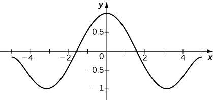
66) [T] Suppose that $\displaystyle \sum_{n=0}^∞a_nx^n$ converges to a function $f(x)$ such that $f(0)=1,\, f′(0)=0$, and $f''(x)=−f(x)$. Find a formula for $a_n$ and plot the partial sum $S_N$ for $N=20$ on $[−5,5].$

Answer

As in the previous problem one obtains $a_n=0$ if $n$ is odd and $a_n=−(n+2)(n+1)a_{n+2}$ if $n$ is even, so $a_0=1$ leads to $a_{2n}=\dfrac{(−1)^n}{(2n)!}$.

67) [T] Suppose that $\displaystyle \sum_{n=0}^∞a_nx^n$ converges to a function $f(x)$ such that $f(0)=0,\; f′(0)=1$, and $f''(x)=−f(x)$. Find a formula for an and plot the partial sum $S_N$ for $N=10$ on $[−5,5]$.

68) Suppose that $\displaystyle \sum_{n=0}^∞a_nx^n$ converges to a function $y$ such that $y''−y′+y=0$ where $y(0)=1$ and $y'(0)=0.$ Find a formula that relates $a_{n+2},\;a_{n+1},$ and an and compute $a_0,...,a_5$.

Answer

$\displaystyle y''=\sum_{n=0}^∞(n+2)(n+1)a_{n+2}x^n$ and $\displaystyle y′=\sum_{n=0}^∞(n+1)a_{n+1}x^n$ so $y''−y′+y=0$ implies that $(n+2)(n+1)a_{n+2}−(n+1)a_{n+1}+a_n=0$ or $a_n=\dfrac{a_{n−1}}{n}−\dfrac{a_{n−2}}{n(n−1)}$ for all $n⋅y(0)=a_0=1$ and $y′(0)=a_1=0,$ so $a_2=\frac{1}{2},\;a_3=\frac{1}{6}\;,a_4=0$, and $a_5=−\frac{1}{120}$.

69) Suppose that $\displaystyle \sum_{n=0}^∞a_nx^n$ converges to a function $y$ such that $y''−y′+y=0$ where $y(0)=0$ and $y′(0)=1$. Find a formula that relates $a_{n+2},\;a_{n+1}$, and an and compute $a_1,...,a_5$.

The error in approximating the integral $\displaystyle ∫^b_af(t)\, dt$ by that of a Taylor approximation $\displaystyle ∫^b_aPn(t) \,dt$ is at most $\displaystyle ∫^b_aR_n(t) \,dt$. In exercises 70 - 71, the Taylor remainder estimate $R_n≤\frac{M}{(n+1)!}|x−a|^{n+1}$ guarantees that the integral of the Taylor polynomial of the given order approximates the integral of $f$ with an error less than $\frac{1}{10}$.

a. Evaluate the integral of the appropriate Taylor polynomial and verify that it approximates the CAS value with an error less than $\frac{1}{100}$.

b. Compare the accuracy of the polynomial integral estimate with the remainder estimate.

70) [T] $\displaystyle ∫^π_0\frac{\sin t}{t}\, dt;\quad P_s=1−\frac{x^2}{3!}+\frac{x^4}{5!}−\frac{x^6}{7!}+\frac{x^8}{9!}$ (You may assume that the absolute value of the ninth derivative of $\frac{\sin t}{t}$ is bounded by $0.1$.)

Answer

a. (Proof)
b. We have $R_s≤\frac{0.1}{(9)!}π^9≈0.0082<0.01.$ We have $\displaystyle ∫^π_0\left(1−\frac{x^2}{3!}+\frac{x^4}{5!}−\frac{x^6}{7!}+\frac{x^8}{9!}\right)\,dx=π−\frac{π^3}{3⋅3!}+\frac{π^5}{5⋅5!}−\frac{π^7}{7⋅7!}+\frac{π^9}{9⋅9!}=1.852...,$ whereas $\displaystyle ∫^π_0\frac{\sin t}{t}\,dt=1.85194...$, so the actual error is approximately $0.00006.$

71) [T] $\displaystyle ∫^2_0e^{−x^2}\,dx;\; p_{11}=1−x^2+\frac{x^4}{2}−\frac{x^6}{3!}+⋯−\frac{x^{22}}{11!}$ (You may assume that the absolute value of the $23^{\text{rd}}$ derivative of $e^{−x^2}$ is less than $2×10^{14}$.)

The following exercises (72-73) deal with Fresnel integrals.

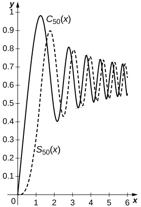
72) The Fresnel integrals are defined by $\displaystyle C(x)=∫^x_0\cos(t^2)\,dt$ and $\displaystyle S(x)=∫^x_0\sin(t^2)\,dt$. Compute the power series of $C(x)$ and $S(x)$ and plot the sums $C_N(x)$ and $S_N(x)$ of the first $N=50$ nonzero terms on $[0,2π]$.

Answer

Since $\displaystyle \cos(t^2)=\sum_{n=0}^∞(−1)^n\frac{t^{4n}}{(2n)!}$ and $\displaystyle \sin(t^2)=\sum_{n=0}^∞(−1)^n\frac{t^{4n+2}}{(2n+1)!}$, one has $\displaystyle S(x)=\sum_{n=0}^∞(−1)^n\frac{x^{4n+3}}{(4n+3)(2n+1)!}$ and $\displaystyle C(x)=\sum_{n=0}^∞(−1)^n\frac{x^{4n+1}}{(4n+1)(2n)!}$. The sums of the first $50$ nonzero terms are plotted below with $C_{50}(x)$ the solid curve and $S_{50}(x)$ the dashed curve.

73) [T] The Fresnel integrals are used in design applications for roadways and railways and other applications because of the curvature properties of the curve with coordinates $(C(t),S(t))$. Plot the curve $(C_{50},S_{50})$ for $0≤t≤2π$, the coordinates of which were computed in the previous exercise.

74) Estimate $\displaystyle ∫^{1/4}_0\sqrt{x−x^2}\,dx$ by approximating $\sqrt{1−x}$ using the binomial approximation $\displaystyle 1−\frac{x}{2}−\frac{x^2}{8}−\frac{x^3}{16}−\frac{5x^4}{2128}−\frac{7x^5}{256}$.

Answer

$\displaystyle ∫^{1/4}_0\sqrt{x}\left(1−\frac{x}{2}−\frac{x^2}{8}−\frac{x^3}{16}−\frac{5x^4}{128}−\frac{7x^5}{256}\right)\,dx =\frac{2}{3}2^{−3}−\frac{1}{2}\frac{2}{5}2^{−5}−\frac{1}{8}\frac{2}{7}2^{−7}−\frac{1}{16}\frac{2}{9}2^{−9}−\frac{5}{128}\frac{2}{11}2^{−11}−\frac{7}{256}\frac{2}{13}2^{−13}=0.0767732...$ whereas $\displaystyle ∫^{1/4}_0\sqrt{x−x^2}\, dx=0.076773.$

75) [T] Use Newton’s approximation of the binomial $\sqrt{1−x^2}$ to approximate $π$ as follows. The circle centered at $(\frac{1}{2},0)$ with radius $\frac{1}{2}$ has upper semicircle $y=\sqrt{x}\sqrt{1−x}$. The sector of this circle bounded by the $x$-axis between $x=0$ and $x=\frac{1}{2}$ and by the line joining $(\frac{1}{4},\frac{\sqrt{3}}{4})$ corresponds to $\frac{1}{6}$ of the circle and has area $\frac{π}{24}$. This sector is the union of a right triangle with height $\frac{\sqrt{3}}{4}$ and base $\frac{1}{4}$ and the region below the graph between $x=0$ and $x=\frac{1}{4}$. To find the area of this region you can write $y=\sqrt{x}\sqrt{1−x}=\sqrt{x}×(\text{binomial expansion of} \sqrt{1−x})$ and integrate term by term. Use this approach with the binomial approximation from the previous exercise to estimate $π$.

76) Use the approximation $T≈2π\sqrt{\frac{L}{g}}(1+\frac{k^2}{4})$ to approximate the period of a pendulum having length $10$ meters and maximum angle $θ_{max}=\frac{π}{6}$ where $k=\sin\left(\frac{θ_{max}}{2}\right)$. Compare this with the small angle estimate $T≈2π\sqrt{\frac{L}{g}}$.

Answer

$T≈2π\sqrt{\frac{10}{9.8}}\left(1+\frac{\sin^2(θ/12)}{4}\right)≈6.453$ seconds. The small angle estimate is $T≈2π\sqrt{\frac{10}{9.8}≈6.347}$. The relative error is around $2$ percent.

77) Suppose that a pendulum is to have a period of $2$ seconds and a maximum angle of $θ_{max}=\frac{π}{6}$. Use $T≈2π\sqrt{\dfrac{L}{g}}\left(1+\dfrac{k^2}{4}\right)$ to approximate the desired length of the pendulum. What length is predicted by the small angle estimate $T≈2π\sqrt{\frac{L}{g}}$?

78) Evaluate $\displaystyle ∫^{π/2}_0\sin^4θ\,dθ$ in the approximation $\displaystyle T=4\sqrt{\frac{L}{g}}∫^{π/2}_0\left(1+\frac{1}{2}k^2\sin^2θ+\frac{3}{8}k^4\sin^4θ+⋯\right)\,dθ$ to obtain an improved estimate for $T$.

Answer

$\displaystyle ∫^{π/2}_0\sin^4θ\, dθ=\frac{3π}{16}.$ Hence $T≈2π\sqrt{\frac{L}{g}}\left(1+\frac{k^2}{4}+\frac{9}{256}k^4\right).$

79) [T] An equivalent formula for the period of a pendulum with amplitude $\displaystyle θ_{max}$ is $T(θ_{max})=2\sqrt{2}\sqrt{\frac{L}{g}}∫^{θ_{max}}_0\frac{dθ}{\sqrt{\cos θ}−\cos(θ_{max})}$ where $L$ is the pendulum length and $g$ is the gravitational acceleration constant. When $θ_{max}=\frac{π}{3}$ we get $\dfrac{1}{\sqrt{\cos t−1/2}}≈\sqrt{2}\left(1+\frac{t^2}{2}+\frac{t^4}{3}+\frac{181t^6}{720}\right)$. Integrate this approximation to estimate $T(\frac{π}{3})$ in terms of $L$ and $g$. Assuming $g=9.806$ meters per second squared, find an approximate length $L$ such that $T(\frac{π}{3})=2$ seconds.

Contributors

Gilbert Strang (MIT) and Edwin “Jed” Herman (Harvey Mudd) with many contributing authors. This content by OpenStax is licensed with a CC-BY-SA-NC 4.0 license. Download for free at http://cnx.org.