3.1: Graphs of Quadratic Functions

Last updated
Save as PDF

Page ID: 141501

\( \newcommand{\vecs}[1]{\overset { \scriptstyle \rightharpoonup} {\mathbf{#1}} } \) \( \newcommand{\vecd}[1]{\overset{-\!-\!\rightharpoonup}{\vphantom{a}\smash {#1}}} \)\(\newcommand{\id}{\mathrm{id}}\) \( \newcommand{\Span}{\mathrm{span}}\) \( \newcommand{\kernel}{\mathrm{null}\,}\) \( \newcommand{\range}{\mathrm{range}\,}\) \( \newcommand{\RealPart}{\mathrm{Re}}\) \( \newcommand{\ImaginaryPart}{\mathrm{Im}}\) \( \newcommand{\Argument}{\mathrm{Arg}}\) \( \newcommand{\norm}[1]{\| #1 \|}\) \( \newcommand{\inner}[2]{\langle #1, #2 \rangle}\) \( \newcommand{\Span}{\mathrm{span}}\) \(\newcommand{\id}{\mathrm{id}}\) \( \newcommand{\Span}{\mathrm{span}}\) \( \newcommand{\kernel}{\mathrm{null}\,}\) \( \newcommand{\range}{\mathrm{range}\,}\) \( \newcommand{\RealPart}{\mathrm{Re}}\) \( \newcommand{\ImaginaryPart}{\mathrm{Im}}\) \( \newcommand{\Argument}{\mathrm{Arg}}\) \( \newcommand{\norm}[1]{\| #1 \|}\) \( \newcommand{\inner}[2]{\langle #1, #2 \rangle}\) \( \newcommand{\Span}{\mathrm{span}}\)\(\newcommand{\AA}{\unicode[.8,0]{x212B}}\)

Learning Objectives

Graph quadratic functions.
Compare graphs of quadratic functions.
Graph quadratic functions in intercept form.
Analyze graphs of real-world quadratic functions.

Introduction

The graphs of quadratic functions are curved lines called parabolas. You don't have to look hard to find parabolic shapes around you. Here ore o few examples:

The path that a ball or a rocket takes through the air.
Water flowing out of a drinking fountain.
The shape of a satellite dish.
The shape of the mirror in car headlights or a flashlight.
The cobles in a suspension bridge.

Graphing Quadratic Functions

Let's see what o porabola looks like by grophing the simplest quadratic function, \(y=x^2\).

We'll graph this function by making a table of values. Since the graph will be curved, we need to plot a fair number of points to make it accurate.

1.1. Graphs of Quadratic Functions

x	y = x²
−3	(−3)² = 9
–2	(−2)² = 4
–1	(−1)² = 1
0	(0)² = 0
1	(1)² = 1
2	(2)² = 4
3	(3)² = 9

Here are the points plotted on a coordinate graph:

f-d:1104d7911634977a8c4c3610d16695eeb521e12740c4c95d7938fd07IMAGE_TINYIMAGE_TINY.1 — Figure \(\PageIndex{1}\)

To draw the parabola, draw a smooth curve through all the points. (Do not connect the points with straight lines).

Let’s graph a few more examples.

Example \(\PageIndex{1}\)

Graph the following parabolas.

y = 2x² + 4x + 1
y = −x² + 3
y = x² − 8x + 3

Solution

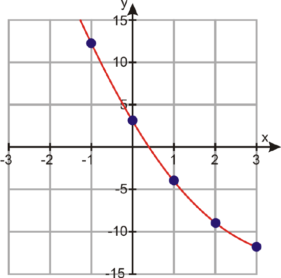
a) y = 2x² + 4x + 1

Make a table of values:

x	y = 2x² + 4x + 1
−3	2(−3)² + 4(−3) + 1 = 7
–2	2(−2)² + 4(−2) + 1 = 1
–1	2(−1)² + 4(−1) + 1 = −1
0	2(0)² + 4(0) + 1 = 1
1	2(1)² + 4(1) + 1 = 7
2	2(2)² + 4(2) + 1 = 17
3	2(3)² + 4(3) + 1 = 31

Notice that the last two points have very large y− values. Since we don’t want to make our y− scale too big, we’ll just skip graphing those two points. But we’ll plot the remaining points and join them with a smooth curve.

b) y = −x² + 3

Make a table of values:

x	y = −x² + 3
−3	−(−3)² + 3 = −6
–2	−(−2)² + 3 = −1
–1	−(−1)² + 3 = 2
0	−(0)² + 3 = 3
1	−(1)² + 3 = 2
2	−(2)² + 3 = −1
3	−(3)² + 3 = −6

Plot the points and join them with a smooth curve.

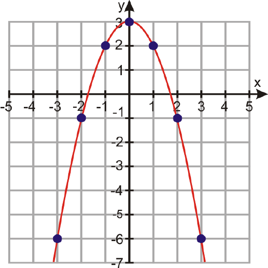
Notice that this time we get an “upside down” parabola. That’s because our equation has a negative sign in front of the x² term. The sign of the coefficient of the x² term determines whether the parabola turns up or down: the parabola turns up if it’s positive and down if it’s negative.

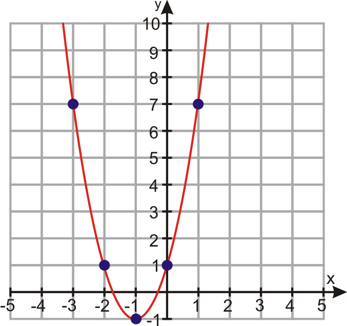
c) y = x² − 8x + 3

Make a table of values:

x	y = x² − 8x + 3
−3	(−3)² − 8(−3) + 3 = 36
–2	(−2)² − 8(−2) + 3 = 23
–1	(−1)² − 8(−1) + 3 = 12
0	(0)² − 8(0) + 3 = 3
1	(1)² − 8(1) + 3 = −4
2	(2)² − 8(2) + 3 = −9
3	(3)² − 8(3) + 3 = −12

Let’s not graph the first two points in the table since the values are so big. Plot the remaining points and join them with a smooth curve.

Wait—this doesn’t look like a parabola. What’s going on here?

Maybe if we graph more points, the curve will look more familiar. For negative values of x it looks like the values of y are just getting bigger and bigger, so let’s pick more positive values of x beyond x = 3 .

x	y = x² − 8x + 3
−1	(−1)² − 8(−1) + 3 = 12
0	(0)² − 8(0) + 3 = 3
1	(1)² − 8(1) + 3 = −4
2	(2)² − 8(2) + 3 = −9
3	(3)² − 8(3) + 3 = −12
4	(4)² − 8(4) + 3 = −13
5	(5)² − 8(5) + 3 = −12
6	(6)² − 8(6) + 3 = −9
7	(7)² − 8(7) + 3 = −4
8	(8)² − 8(8) + 3 = 3

Plot the points again and join them with a smooth curve.

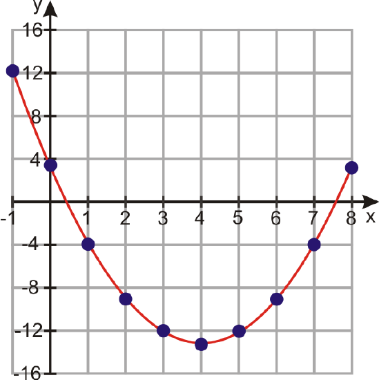
Now we can see the familiar parabolic shape. And now we can see the drawback to graphing quadratics by making a table of values—if we don’t pick the right values, we won’t get to see the important parts of the graph.

In the next couple of lessons, we’ll find out how to graph quadratic equations more efficiently—but first we need to learn more about the properties of parabolas.

Compare Graphs of Quadratic Functions

The general form (or standard form) of a quadratic function is:

y = ax² + bx + c

Here a, b and c are the coefficients. Remember, a coefficient is just a number (a constant term) that can go before a variable or appear alone.

Although the graph of a quadratic equation in standard form is always a parabola, the shape of the parabola depends on the values of the coefficients a, b and c. Let’s explore some of the ways the coefficients can affect the graph

Dilation

Changing the value of a makes the graph “fatter” or “skinnier”. Let’s look at how graphs compare for different positive values of a . The plot on the left shows the graphs of

\(y =x^2\) and \(y=3x^2\). The plot on the right shows the graphs of \(y =x^2\) and\( \dfrac{1}{3} x^2 \)

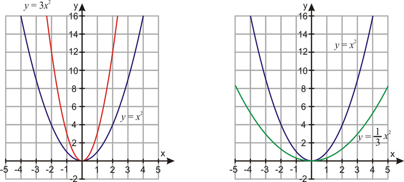
Notice that the larger the value of a is, the skinnier the graph is – for example, in the first plot, the graph of \(y=3x^2\) is skinnier than the graph of \(y=x^2\). Also, the smaller a is, the fatter the graph is – for example, in the second plot, the graph of \(y=dfrac{1}{3}x^2\) is fatter than the graph of \(y=x^2\). This might seem counterintuitive, but if you think about it, it should make sense. Let’s look at a table of values of these graphs and see if we can explain why this happens.

\(x\)	\(y=x^2\)	\(y=3x^2\)	\(y=dfrac{1}{3}x^2\)
−3	(−3)² = 9	3(−3)² = 27	\(dfrac{-3^2}{3}=3\)
–2	(−2)² = 4	3(−2)² = 12	\(dfrac{-2^2}{3}=dfrac{4}{3}\)
–1	(−1)² = 1	3(−1)² = 3	\(dfrac{-1^2}{3}=dfrac{1}{3}\)
0	(0)² = 0	3(0)² = 0	\(dfrac{-0^2}{3}=0\)
1	(1)² = 1	3(1)² = 3	\(dfrac{1^2}{3}=dfrac{1}{3}\)
2	(2)² = 4	3(2)² = 12	\(dfrac{2^2}{3}=dfrac{4}{3}\)
3	(3)² = 9	3(3)² = 27	\(dfrac{3^2}{3}=3

From the table, you can see that the values of \(y=3x^2\) are bigger than the values of \(y=x^2\). This is because each value of y gets multiplied by 3. As a result the parabola will be skinnier because it grows three times faster than \(y=3x^2\). On the other hand, you can see that the values of \(y=dfrac{1}{3}x^2\) are smaller than the values of \(y=x^2\), because each value of y gets divided by 3. As a result the parabola will be fatter because it grows at one third the rate of \(y=x^2\).

Orientation

As the value of a gets smaller and smaller, then, the parabola gets wider and flatter. What happens when a gets all the way down to zero? What happens when it’s negative?

Well, when a=0, the \(x^2\) term drops out of the equation entirely, so the equation becomes linear and the graph is just a straight line. For example, we just saw what happens to \(y=ax^2\) when we change the value of a; if we tried to graph \(y=0x^2\), we would just be graphing y=0, which would be a horizontal line.

So as a gets smaller and smaller, the graph of \(y=ax^2\) gets flattened all the way out into a horizontal line. Then, when a becomes negative, the graph of \(y=ax^2\) starts to curve again, only it curves downward instead of upward. This fits with what you’ve already learned: the graph opens upward if a is positive and downward if a is negative.

For example, here are the graphs of \(y=ax^2\) and \(y=-ax^2\). You can see that the parabola has the same shape in both graphs, but the graph of \(y=ax^2\) is right-side-up and the graph of \(y=-ax^2\) is upside-down.

Vertical Shift

Changing the constant c just shifts the parabola up or down. The following plot shows the graphs of \(y=x^2, y=x^2+1, y=x^2-1, y=x^2+2\), and \(y=x^2-2\)

You can see that when c is positive, the graph shifts up, and when c is negative the graph shifts down; in either case, it shifts by |c| units. In one of the later sections we’ll learn about horizontal shift (i.e. moving to the right or to the left). Before we can do that, though, we need to learn how to rewrite quadratic equations in different forms.

Meanwhile, if you want to explore further what happens when you change the coefficients of a quadratic equation, the page at http://www.analyzemath.com/quadraticg/quadraticg.htm has an applet you can use. Click on the “Click here to start” button in section A, and then use the sliders to change the values of a,b, and c.

Graph Quadratic Functions in Intercept Form

Now it’s time to learn how to graph a parabola without having to use a table with a large number of points.

Let’s look at the graph of \(y=x^2−6x+8\).

f-d:70c8a98694d06f8f8b625330c6af75f9e53ad29201bcedcbfbe61d1bIMAGE_TINYIMAGE_TINY.1 — Figure \(\PageIndex{10}\)

There are several things we can notice:

The parabola crosses the x−axis at two points: x=2 and x=4. These points are called the x− intercepts of the parabola.
The lowest point of the parabola occurs at (3, -1).
- This point is called the vertex of the parabola.
- The vertex is the lowest point in any parabola that turns upward, or the highest point in any parabola that turns downward.
- The vertex is exactly halfway between the two x−intercepts. This will always be the case, and you can find the vertex using that property.
The parabola is symmetric. If you draw a vertical line through the vertex, you see that the two halves of the parabola are mirror images of each other. This vertical line is called the line of symmetry.

We said that the general form of a quadratic function is y=ax2+bx+c. When we can factor a quadratic expression, we can rewrite the function in intercept form:

\(y=a(x−m)(x−n)\)

This form is very useful because it makes it easy for us to find the x−intercepts and the vertex of the parabola. The x−intercepts are the values of x where the graph crosses the x−axis; in other words, they are the values of x when y=0. To find the x−intercepts from the quadratic function, we set y=0 and solve:

\[0=a(x-m)(x-n)\]
Since the equation is already factored, we use the zero-product property to set each factor equal to zero and solve the individual linear equations:
\[\begin{aligned}
x-m & =0 & & x-n & =0 \\
x & \text { or } & & x & =n
\end{aligned}\]

So the \(x\)-intercepts are at points \((m, 0)\) and \((n, 0)\).
Once we find the \(x\)-intercepts, it's simple to find the vertex. The \(x\) value of the vertex is halfway between the two \(x\)-intercepts, so we can find it by taking the average of the two values: \(\frac{m+n}{2}\). Then we can find the \(y\)-value by plugging the value of \(x\) back into the equation of the function.

Example \(\PageIndex{2}\)

Find the \(x\)-intercepts and the vertex of the following quadratic functions:

a) \(y=x^2-8 x+15\)
b) \(y=3 x^2+6 x-24\)

Solution

a) \(y=x^2-8 x+15\)

Write the quadratic function in intercept form by factoring the right hand side of the equation. Remember, to factor we need two numbers whose product is 15 and whose sum is -8 . These numbers are -5 and -3 .

The function in intercept form is \(y=(x-5)(x-3)\)

We find the \(x\)-intercepts by setting \(y=0\).

We have:
\[
\begin{array}{lll}
0=(x-5)(x-3) & & \\
x-5=0 & \text { or } & \\
& & x-3=0 \\
x=5 & & x=3
\end{array}
\]

So the \(x\)-intercepts are \((5,0)\) and \((3,0)\).

The vertex is halfway between the two \(x\)-intercepts. We find the \(x-\) value by taking the average of the two \(x\)-intercepts: \(x=\frac{5+3}{2}=4\)
We find the \(y\)-value by plugging the \(x\)-value we just found into the original equation:
\[
y=x^2-8 x+15 \Rightarrow y=4^2-8(4)+15=16-32+15=-1
\]
So the vertex is \((4,-1)\).

b) \(y=3 x^2+6 x-24\)
Re-write the function in intercept form.

Factor the common term of 3 first: \(y=3\left(x^2+2 x-8\right)\)

Then factor completely: \(y=3(x+4)(x-2)\)

Set \(y=0\) and solve:
\[
\begin{array}{l}
x+4=0 \\
x-2=0 \\
0=3(x+4)(x-2) \Rightarrow \\
x=-4 \\
x=2 \\
\end{array}
\]

The \(x\)-intercepts are \((-4,0)\) and \((2,0)\).

For the vertex,
\[
\begin{array}{l}
x=\frac{-4+2}{2}=-1 \text { and } \\
y=3(-1)^2+6(-1)-24=3-6-24=-27
\end{array}
\]

The vertex is: \((-1,-27)\)

Knowing the vertex and \(x\)-intercepts is a useful first step toward being able to graph quadratic functions more easily. Knowing the vertex tells us where the middle of the parabola is. When making a table of values, we can make sure to pick the vertex as a point in the table. Then we choose just a few smaller and larger values of \(x\). In this way, we get an accurate graph of the quadratic function without having to have too many points in our table.

Example \(\PageIndex{3}\)

Find the \(x\)-intercepts and vertex. Use these points to create a table of values and graph each function.

a) \(y=x^2-4\)
b) \(y=-x^2+14 x-48\)

Solution

a) \(y=x^2-4\)

Let's find the \(x\)-intercepts and the vertex:

Factor the right-hand side of the function to put the equation in intercept form:
\[
y=(x-2)(x+2)
\]
Set \(y=0\) and solve:
\[
\begin{array}{lll}
0=(x-2)(x+2) & & \\
x-2=0 & \text { or } & \\
& & x+2=0 \\
x=2 & & x=-2
\end{array}
\]

The \(x\)-intercepts are \((2,0)\) and \((-2,0)\).

Find the vertex:
\[
x=\frac{2-2}{2}=0 \quad y=(0)^2-4=-4
\]
The vertex is \((0,-4)\).

Make a table of values using the vertex as the middle point. Pick a few values of \(x\) smaller and larger than \(x=0\). Include the \(x\)-intercepts in the table.

x y = x² − 4
−3	y = (−3)² − 4 = 5
–2	y = (−2)² − 4 = 0	x− intercept
–1	y = (−1)² − 4 = −3
0	y = (0)² − 4 = −4	vertex
1	y = (1)² − 4 = −3
2	y = (2)² − 4 = 0	x− intercept
3	y = (3)² − 4 = 5

Then plot the graph:

b) \(y=-x^2+14 x-48\)

Let's find the \(x\)-intercepts and the vertex:

Factor the right-hand-side of the function to put the equation in intercept form:
\[
y=-\left(x^2-14 x+48\right)=-(x-6)(x-8)
\]
Set \(y=0\) and solve:
\[
\begin{array}{lll}
0=-(x-6)(x-8) & & \\
x-6=0 & & x-8=0 \\
x=6 & \text { or } & \\
x=8
\end{array}
\]

The \(x\)-intercepts are \((6,0)\) and \((8,0)\).

Find the vertex:
\[
x=\frac{6+8}{2}=7 \quad y=-(7)^2+14(7)-48=1
\]
The vertex is \((7,1)\).

Make a table of values using the vertex as the middle point. Pick a few values of \(x\) smaller and larger than \(x=7\). Include the \(x\)-intercepts in the table.

x	y = −x² + 14x − 48
4	y = −(4)² + 14(4) − 48 = −8
5	y = −(5)² + 14(5) − 48 = −3
6	y = −(6)² + 14(6) − 48 = 0
7	y = −(7)² + 14(7) − 48 = 1
8	y = −(8)² + 14(8) − 48 = 0
9	y = −(9)² + 14(9) − 48 = −3
10	y = −(10)² + 14(10) − 48 = −8

Then plot the graph:

Analyze Graphs of Real-World Quadratic Functions.

As we mentioned at the beginning of this section, parabolic curves are common in real- world applications. Here we will look at a few graphs that represent some examples of real- life application of quadratic functions.

Example \(\PageIndex{4}\)

Andrew has 100 feet of fence to enclose a rectangular tomato patch. What should the dimensions of the rectangle be in order for the rectangle to have the greatest possible area?

Solution

f-d:5596c58f69f8ed41a05d29e4664eb5dc7ac3d4c17cacfffc714b9099IMAGE_TINYIMAGE_TINY.1 — Figure \(\PageIndex{13}\)

If the length of the rectangle is \(x\), then the width is \(50-x\). (The length and the width add up to 50 , not 100 , because two lengths and two widths together add up to 100.)

If we let \(y\) be the area of the triangle, then we know that the area is length \(\times\) width, so \(y=x(50-x)=50 x-x^2\).

Here's the graph of that function, so we can see how the area of the rectangle depends on the length of the rectangle:

We can see from the graph that the highest value of the area occurs when the length of the rectangle is 25 . The area of the rectangle for this side length equals 625. (Notice that the width is also 25, which makes the shape a square with side length 25 .)

This is an example of an optimization problem. These problems show up often in the real world, and if you ever study calculus, you'll learn how to solve them without graphs.

Example \(\PageIndex{5}\)

Anne is playing golf. On the \(4^{\text {th }}\) tee, she hits a slow shot down the level fairway. The ball follows a parabolic path described by the equation \(y=x-0.04 x^2\), where \(y\) is the ball's height in the air and \(x\) is the horizontal distance it has traveled from the tee. The distances are measured in feet. How far from the tee does the ball hit the ground? At what distance from the tee does the ball attain its maximum height? What is the maximum height?

Solution

Let's graph the equation of the path of the ball:

\(x(1-0.04 x)=0\) has solutions \(x=0\) and \(x=25\).

From the graph, we see that the ball hits the ground \(\mathbf{2 5}\) feet from the tee. (The other \(x\)-intercept, \(x=0\), tells us that the ball was also on the ground when it was on the tee!)

We can also see that the ball reaches its maximum height of about 6.25 feet when it is \(\mathbf{1 2 . 5}\) feet from the tee.

Review Questions

Rewrite the following functions in intercept form. Find the \(x\)-intercepts and the vertex.
1. \(y=x^2-2 x-8\)
2. \(y=-x^2+10 x-21\)
3. \(y=2 x^2+6 x+4\)
4. \(y=3(x+5)(x-2)\)

Does the graph of the parabola turn up or down?
5. \(y=-2 x^2-2 x-3\)
6. \(y=3 x^2\)
7. \(y=16-4 x^2\)
8. \(y=3 x^2-2 x-4 x^2+3\)

The vertex of which parabola is higher?
9. \(y=x^2+4\) or \(y=x^2+1\)
10. \(y=-2 x^2\) or \(y=-2 x^2-2\)
11. \(y=3 x^2-3\) or \(y=3 x^2-6\)
12. \(y=5-2 x^2\) or \(y=8-2 x^2\)

Which parabola is wider?
13. \(y=x^2\) or \(y=4 x^2\)
14. \(y=2 x^2+4\) or \(y=\frac{1}{2} x^2+4\)
15. \(y=-2 x^2-2\) or \(y=-x^2-2\)
16. \(y=x^2+3 x^2\) or \(y=x^2+3\)

Graph the following functions by making a table of values. Use the vertex and \(x\)-intercepts to help you pick values for the table.
17. \(y=4 x^2-4\)
18. \(y=-x^2+x+12\)
19. \(y=2 x^2+10 x+8\)
20. \(y=\frac{1}{2} x^2-2 x\)
21. \(y=x-2 x^2\)
22. \(y=4 x^2-8 x+4\)

23. Nadia is throwing a ball to Peter. Peter does not catch the ball and it hits the ground. The graph shows the path of the ball as it flies through the air. The equation that describes the path of the ball is \(y=4+2 x-0.16 x^2\). Here \(y\) is the height of the ball and \(x\) is the horizontal distance from Nadia. Both distances are measured in feet.
a. How far from Nadia does the ball hit the ground?
b. At what distance \(x\) from Nadia, does the ball attain its maximum height?
c. What is the maximum height?

24. Jasreel wants to enclose a vegetable patch with 120 feet of fencing. He wants to put the vegetable against an existing wall, so he only needs fence for three of the sides. The equation for the area is given by \(A=120 x-x^2\). From the graph, find what dimensions of the rectangle would give him the greatest area.