
4.2 Graphing Functions With Transformations
- Page ID
- 153537

\( \newcommand{\vecs}[1]{\overset { \scriptstyle \rightharpoonup} {\mathbf{#1}} } \)
\( \newcommand{\vecd}[1]{\overset{-\!-\!\rightharpoonup}{\vphantom{a}\smash {#1}}} \)
\( \newcommand{\dsum}{\displaystyle\sum\limits} \)
\( \newcommand{\dint}{\displaystyle\int\limits} \)
\( \newcommand{\dlim}{\displaystyle\lim\limits} \)
\( \newcommand{\id}{\mathrm{id}}\) \( \newcommand{\Span}{\mathrm{span}}\)
( \newcommand{\kernel}{\mathrm{null}\,}\) \( \newcommand{\range}{\mathrm{range}\,}\)
\( \newcommand{\RealPart}{\mathrm{Re}}\) \( \newcommand{\ImaginaryPart}{\mathrm{Im}}\)
\( \newcommand{\Argument}{\mathrm{Arg}}\) \( \newcommand{\norm}[1]{\| #1 \|}\)
\( \newcommand{\inner}[2]{\langle #1, #2 \rangle}\)
\( \newcommand{\Span}{\mathrm{span}}\)
\( \newcommand{\id}{\mathrm{id}}\)
\( \newcommand{\Span}{\mathrm{span}}\)
\( \newcommand{\kernel}{\mathrm{null}\,}\)
\( \newcommand{\range}{\mathrm{range}\,}\)
\( \newcommand{\RealPart}{\mathrm{Re}}\)
\( \newcommand{\ImaginaryPart}{\mathrm{Im}}\)
\( \newcommand{\Argument}{\mathrm{Arg}}\)
\( \newcommand{\norm}[1]{\| #1 \|}\)
\( \newcommand{\inner}[2]{\langle #1, #2 \rangle}\)
\( \newcommand{\Span}{\mathrm{span}}\) \( \newcommand{\AA}{\unicode[.8,0]{x212B}}\)
\( \newcommand{\vectorA}[1]{\vec{#1}} % arrow\)
\( \newcommand{\vectorAt}[1]{\vec{\text{#1}}} % arrow\)
\( \newcommand{\vectorB}[1]{\overset { \scriptstyle \rightharpoonup} {\mathbf{#1}} } \)
\( \newcommand{\vectorC}[1]{\textbf{#1}} \)
\( \newcommand{\vectorD}[1]{\overrightarrow{#1}} \)
\( \newcommand{\vectorDt}[1]{\overrightarrow{\text{#1}}} \)
\( \newcommand{\vectE}[1]{\overset{-\!-\!\rightharpoonup}{\vphantom{a}\smash{\mathbf {#1}}}} \)
\( \newcommand{\vecs}[1]{\overset { \scriptstyle \rightharpoonup} {\mathbf{#1}} } \)
\(\newcommand{\longvect}{\overrightarrow}\)
\( \newcommand{\vecd}[1]{\overset{-\!-\!\rightharpoonup}{\vphantom{a}\smash {#1}}} \)
\(\newcommand{\avec}{\mathbf a}\) \(\newcommand{\bvec}{\mathbf b}\) \(\newcommand{\cvec}{\mathbf c}\) \(\newcommand{\dvec}{\mathbf d}\) \(\newcommand{\dtil}{\widetilde{\mathbf d}}\) \(\newcommand{\evec}{\mathbf e}\) \(\newcommand{\fvec}{\mathbf f}\) \(\newcommand{\nvec}{\mathbf n}\) \(\newcommand{\pvec}{\mathbf p}\) \(\newcommand{\qvec}{\mathbf q}\) \(\newcommand{\svec}{\mathbf s}\) \(\newcommand{\tvec}{\mathbf t}\) \(\newcommand{\uvec}{\mathbf u}\) \(\newcommand{\vvec}{\mathbf v}\) \(\newcommand{\wvec}{\mathbf w}\) \(\newcommand{\xvec}{\mathbf x}\) \(\newcommand{\yvec}{\mathbf y}\) \(\newcommand{\zvec}{\mathbf z}\) \(\newcommand{\rvec}{\mathbf r}\) \(\newcommand{\mvec}{\mathbf m}\) \(\newcommand{\zerovec}{\mathbf 0}\) \(\newcommand{\onevec}{\mathbf 1}\) \(\newcommand{\real}{\mathbb R}\) \(\newcommand{\twovec}[2]{\left[\begin{array}{r}#1 \\ #2 \end{array}\right]}\) \(\newcommand{\ctwovec}[2]{\left[\begin{array}{c}#1 \\ #2 \end{array}\right]}\) \(\newcommand{\threevec}[3]{\left[\begin{array}{r}#1 \\ #2 \\ #3 \end{array}\right]}\) \(\newcommand{\cthreevec}[3]{\left[\begin{array}{c}#1 \\ #2 \\ #3 \end{array}\right]}\) \(\newcommand{\fourvec}[4]{\left[\begin{array}{r}#1 \\ #2 \\ #3 \\ #4 \end{array}\right]}\) \(\newcommand{\cfourvec}[4]{\left[\begin{array}{c}#1 \\ #2 \\ #3 \\ #4 \end{array}\right]}\) \(\newcommand{\fivevec}[5]{\left[\begin{array}{r}#1 \\ #2 \\ #3 \\ #4 \\ #5 \\ \end{array}\right]}\) \(\newcommand{\cfivevec}[5]{\left[\begin{array}{c}#1 \\ #2 \\ #3 \\ #4 \\ #5 \\ \end{array}\right]}\) \(\newcommand{\mattwo}[4]{\left[\begin{array}{rr}#1 \amp #2 \\ #3 \amp #4 \\ \end{array}\right]}\) \(\newcommand{\laspan}[1]{\text{Span}\{#1\}}\) \(\newcommand{\bcal}{\cal B}\) \(\newcommand{\ccal}{\cal C}\) \(\newcommand{\scal}{\cal S}\) \(\newcommand{\wcal}{\cal W}\) \(\newcommand{\ecal}{\cal E}\) \(\newcommand{\coords}[2]{\left\{#1\right\}_{#2}}\) \(\newcommand{\gray}[1]{\color{gray}{#1}}\) \(\newcommand{\lgray}[1]{\color{lightgray}{#1}}\) \(\newcommand{\rank}{\operatorname{rank}}\) \(\newcommand{\row}{\text{Row}}\) \(\newcommand{\col}{\text{Col}}\) \(\renewcommand{\row}{\text{Row}}\) \(\newcommand{\nul}{\text{Nul}}\) \(\newcommand{\var}{\text{Var}}\) \(\newcommand{\corr}{\text{corr}}\) \(\newcommand{\len}[1]{\left|#1\right|}\) \(\newcommand{\bbar}{\overline{\bvec}}\) \(\newcommand{\bhat}{\widehat{\bvec}}\) \(\newcommand{\bperp}{\bvec^\perp}\) \(\newcommand{\xhat}{\widehat{\xvec}}\) \(\newcommand{\vhat}{\widehat{\vvec}}\) \(\newcommand{\uhat}{\widehat{\uvec}}\) \(\newcommand{\what}{\widehat{\wvec}}\) \(\newcommand{\Sighat}{\widehat{\Sigma}}\) \(\newcommand{\lt}{<}\) \(\newcommand{\gt}{>}\) \(\newcommand{\amp}{&}\) \(\definecolor{fillinmathshade}{gray}{0.9}\)By the end of this section, you will be able to:
- grasp the relationship between a function and its graph
- assess whether a graph is the graph of a function using the Vertical Line Test
- sketch graphs of functions
- identify the effect of transformations of functions on their graphs
- identify even and odd functions
A graph is a diagram drawn on a coordinate plane showing the relationship between two variables, each of which is measured along an axis. We've already seen the graphs of lines and circles in detail when learning about equations. Since functions also describe relationships between two variables, an independent input variable and a dependent output variable, we have been able to sketch the graph of a function, essentially drawing on a plane all of the points whose coordinates are related via that function. All functions can be graphed (in some way, although maybe not prettily), but not all graphs represent functions! Let's talk about that.
Vertical Line Test
We saw this graph in the last section:

Here we have the set of infinitely many points that lie on that straight line, whose equation we would recognize as \(y = x+3\). This the graph of the function \( f(x) = x+3\), because at each input \(x\)-value, that function \(f\) will spit out the correct output value for the \(y\)-coordinate. Now consider this graph:
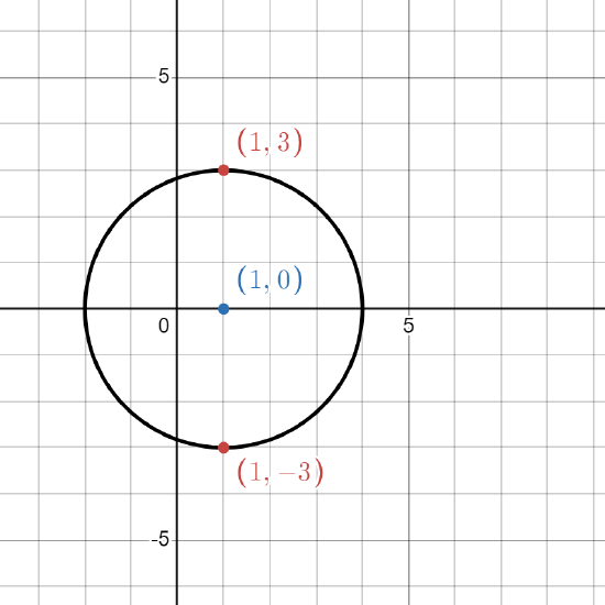
Could this graph be representing a function? Aka, could the \(y\)-coordinates of points on this circle be defined by function values given the \(x\)-coordinates as inputs? I highlighted two points on the circle there. Notice that they both have the \(x\)-coordinate \(1\), and yet they have two distinct \(y\)-coordinates... A function is only allowed to assign one output to each input, so this cannot be the graph of a function! There's a handy trick for assessing this at a glance.
If there is any place on a given graph where you could draw a vertical line that intersects the graph at multiple distinct points, then the graph cannot be the graph of a function.
A vertical line has an equation of the form \(x = a\) and is passing through all the points with \(x\)-coordinate \(a\). If it crosses a graph more than once, that means the graph has multiple \(y\)-values assigned to the same \(x\)-value. Illegal for functions!

Tell whether the following graphs could represent functions.

Solution
The first passes the VLT, as you can draw a vertical line anywhere and have only one intersection, so it represents a linear function. The second is the graph of a hyperbola and fails the VLT, so no.

Tell whether the graphs could represent functions.

- Answer
-
Yes, no, and yes. VLT demonstrated below.

Domain and Range via Graphs
Recall that the domain of a function is its set of inputs (most often, all real numbers that are legal to use as inputs). The range of a function is the set of real numbers that it actually produces as outputs. So like, I could think of the function \(f(x) = x^2\) as taking real numbers and inputs and giving real numbers as outputs, which is certainly true, but more specifically, \(f\) will only give nonnegative real numbers as outputs. Let's look at the graph of this function.

The arms of this parabola continue forever upward and outward. In regard to the \(x\)-axis, all input \(x\)-values are allowed in the domain. But looking at the \(y\)-axis, we see that the graph never passes below the height \(y = 0\). This graph never attains any negative \(y\)-values, but it does attain all positive \(y\)-values as the arms go up and up forever. For this function, the domain is all real numbers, and the range is real numbers \(y\geq 0 \).
Assess the domain and range of the following graphed functions.

Solution
On the left, we see that the function's graph heads down and to the left forever, which means all negative \(x\)- and \(y\)-values can be attained, and up and to the right forever, which means all positive \(x\)- and \(y\)-values can be attained. We know that \(f(x) = x^3\) can take any real number as input, and will give as outputs both positive and negative real numbers. Both the domain and range for this function are \( \mathbb{R}\), all real numbers.
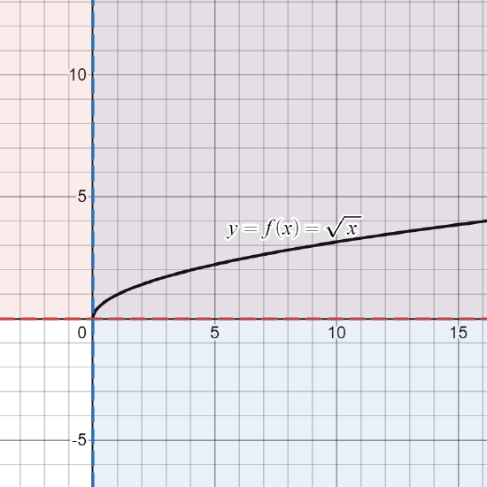
On the right, we see that the graph doesn't appear in the left half of the 2D plane, so it is not defined for any negative \(x\)-values. The graph also stays above the \(x\)-axis forever, meaning it never attains negative \(y\)-values. The domain here is \( \{ x \: | \: x \geq 0\} \) and the range is \( \{y \: | \: y \geq 0\} \).
Transformations of Graphs
Suppose I have a graph of some function like the one given below.

To every single point \( (x,y)\) on the graph, I perform a little operation by adding 2 to the \(y\)-value. This has the effect of scootching each point exactly two units upward. The entire graph appears to have shifted vertically upward by 2, without otherwise changing the shape of the graph.

If this was the graph of a function, \(y = f(x)\), then the new blue line is the graph \(y = f(x) + 2 \). There are several different little transformations you can apply to an original function whose graphical consequences are easy to predict, just like this. I'm going to give you a big table here, but it's important that you read through line by line and understand as much as possible why each operation causes the indicated graph change. Each transformation starts with an original function \(f(x)\) and makes a change to it like \(f(x) + 2\) to produce a new function, which you'll find in the second column.
| Transformation Description | \(f (x) \rightarrow \) New Function | English Translation | Example | Graph |
| Vertical shift up by \(k\) | \( f(x) + k\) | An original function gets a positive constant added on to the very end, which causes a vertical change. |
\(f(x) = x^2, \rightarrow \) \( g(x) = x^2 + 1 \) |
 |
| Vertical shift down by \(k\) | \( f(x) - k \) | An original function gets a constant subtracted on the very end, which causes a vertical change. | \(f(x) = x^2, \rightarrow \) \( g(x) = x^2 - 1 \) |  |
| Horizontal shift right by \(h\) | \( f(x-h) \) | In an original function, each instance of the variable was replaced by the variable minus a constant, causing a horizontal change. | \( f(x) = x^2, \rightarrow \) \( g(x) = (x-1)^2 \) |  |
| Horizontal shift left by \( h\) | \( f(x+h) \) | In an original function, each instance of the variable was replaced by the variable plus a constant, causing a horizontal change. | \( f(x) = x^2, \rightarrow \) \( g(x) = (x+1)^2 \) |  |
| Reflection across the \(x\)-axis | \( - f(x) \) | Flip the sign on the whole original function, which has the effect of flipping the sign on all \(y\)-values. | \( f(x) = x^2, \rightarrow \) \( g(x) = - x^2 \) |  |
| Reflection across the \( y\)-axis | \( f( -x)\) | In an original function, each instance of the variable \(x\) was replaced by \( (-x)\). | \( f(x) = x^3, \rightarrow \) \( g(x) = (-x)^3 \) |  |
| Vertical stretch by a factor of \(k\) | \( k \cdot f(x),\) where \( k > 1 \) | An entire original function is multiplied by a constant larger than 1, causing a vertical change. | \( f(x) = x^3-x, \rightarrow \) \( g(x) = 3(x^3-x) \) | 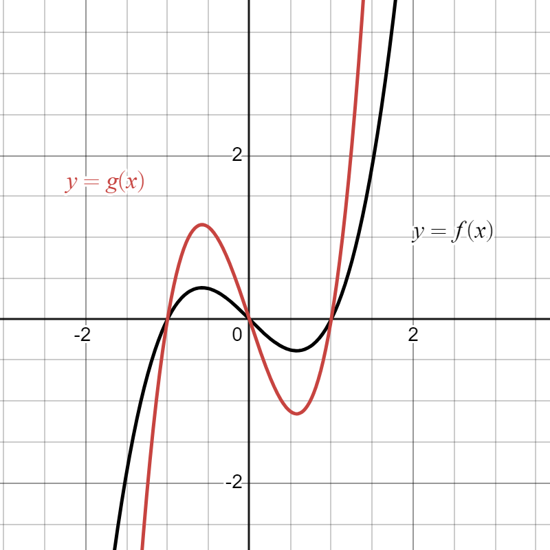 |
| Vertical shrink by a factor of \(k\) | \( k \cdot f(x)\), where \( 0 < k < 1 \) | An entire original function is multiplied by a positive fraction smaller than 1, causing a vertical change. | \(f(x) = x^3-x, \rightarrow \) \(g(x) = \frac{1}{2}(x^3-x) \) |  |
| Horizontal stretch by a factor of \(\frac{1}{h}\) | \( f( hx) \), where \(0 < h < 1 \) | In an original function, each instance of \(x\) is replaced by \(x\) times a small positive fraction, causing a horizontal change. | \( f(x) = x^3-x, \rightarrow \) \( g(x) = (\frac{1}{2}x)^3 - \frac{1}{2}x \) |  |
| Horizontal shrink by a factor of \(\frac{1}{h}\) | \( f(hx)\), where \( h > 1 \) | In an original function, each instance of \(x\) is replaced by \(x\) times a constant larger than 1, causing a horizontal change. | \( f(x) = x^3 - x, \rightarrow \) \( g(x) = (2x)^3-2x \) |  |
All of these transformation types can be combined one after another. When describing this process, sometimes the order in which you perform transformations really matters! See the example below.
Describe the transformation(s) done to \( f(x) = x^3 - x \) to produce the following functions.
- \( g(x) = 2x^3 - 2x \)
- \( g(x) = 8x^3 - 2x \)
- \( g(x) = (x-2)^3 - x + 2 \)
- \( g(x) = (x+1)^3 - x - 3 \)
- \( g(x) = 4(x^3 - x ) + 1 \)
- \( g(x) = -2( (x-1)^3 - (x-1)) \)
Solution
1. We can see that this \(g\) was made by taking \(f (x)\) and multiplying the whole thing by a 2, so \(g(x) = 2f(x) \). According to the table, this causes a vertical stretch by a factor of 2. On the graph, this looks like...

2. This one is slightly different, but if we consider that \(8 = 2^3\), we can see that \(g(x) = f(2x) \). If you go through \(f\) and replace each \(x\) with \((2x)\), you get \(g\). This causes a horizontal change, and since \(2 > 1\), we are looking at a horizontal shrink by a factor of \(\frac{1}{2} \).

3. In this one, we notice that \( (x-h)\) type expression and ask ourselves if this could be a horizontal shift. With a little algebra, we can see that \(g(x) = (x-2)^3 - (x-2) = f(x-2) \). This gives us a horizontal shift to the right by 2.

4. We see that \( (x+h) \) expression and try to do the same algebra trick to see a horizontal shift situation, but we get \( g(x) = (x+1)^3 - (x+1) - 2 \). Well that's okay, we just have a two transformations going on here. First, a horizontal shift left by 1, and then a vertical shift down by 2.
\[ f(x) = x^3 - x \quad \longrightarrow \quad f(\textcolor{blue}{x+1}) = (\textcolor{blue}{x+1})^3 - (\textcolor{blue}{x+1}) \quad \longrightarrow f(x+1) \textcolor{red}{- 2} = (x+1)^3 - (x+1) \textcolor{red}{- 2} = g(x) \notag \]
In the graph below, the "intermediate" step after just the horizontal shift is shown in blue.

5. This one looks like multiple steps again. We get \(g\) by taking \(f\), multiplying it as a whole by 4, and then adding a 1. This means a vertical stretch by a factor of 4, followed by a vertical shift up by 1.
\[ f(x) = x^3 - x \quad \longrightarrow \quad \textcolor{blue}{4 f(x) = 4(x^3 - x)} \quad \longrightarrow \quad \textcolor{red}{4 f(x) +1 = 4(x^3 - x) +1 = g(x) } \notag \]

6. We pick this apart from the inside out as well. The \( (x-h) \) expressions are clues for a horizontal shift to the right. Then the entire result was multiplied by 2, causing a vertical stretch.
\[ f(x) = x^3 - x \quad \longrightarrow \quad \textcolor{blue}{f(x-1) = (x-1)^3 - (x-1)} \quad \longrightarrow \quad \textcolor{green}{2 f(x-1) = 2( (x-1)^3 - (x-1) )} \notag \]
Finally, the entire result was made negative, which causes a reflection over the \( x\)-axis.
\[\cdots \longrightarrow \quad \textcolor{red}{-2f(x-1) = -2( (x-1)^3 - (x-1)) = g(x)} \notag \]

Describe the transformation(s) performed on \( f(x) = \sqrt{x} \) to produce the following functions. If desired, graph both functions using Desmos to reinforce your answers like I did above.
- \( g(x) = \sqrt{x+2} \)
- \( g(x) = 4\sqrt{x} \)
- \( g(x) = -2 \sqrt{x-1} \)
- \( g(x) = \sqrt{-x} + 3 \)
- \( g(x) = \sqrt{ \frac{1}{2} x - 1 } \)
- Answer
-
- Horizontal shift to the left by 2.
- Vertical stretch by a factor of 4.
- Horizontal shift to the right by 1, then vertical stretch by 2, then reflection over the \(x\)-axis.
- Reflection over the \(y\)-axis, then vertical shift up by 3.
- Horizontal shift right by 1, THEN horizontal stretch by a factor of 2. Watch out, if you mix up the order, you will get a different function!
\[ \sqrt{x} \: \longrightarrow \: \sqrt{ \frac{1}{2}x } \: \longrightarrow \: \sqrt{ \frac{1}{2}(x-1)} \quad \neq \quad \sqrt{x} \: \longrightarrow \: \sqrt{x-1} \: \longrightarrow \: \sqrt{ \frac{1}{2}x - 1 } \notag \]
Describe the transformation(s) applied to the black graph to produce the red graph. Hint: pick a point or two and try to see how they in particular moved and changed. Write the formula for \(g(x)\) depending on \(f (x)\).
 |
 |
 |
 |
| 1. | 2. | 3. | 4. |
- Answer
-
- Horizontal shift to the left by 3 (look at the right endpoint, who was at an \(x\)-value of 3 but is now at an \(x\)-value of 0. We have \(g(x) = f(x+3) \).
- Reflection across the \(y\)-axis. We have \(g(x) = f(-x) \).
- Vertical shrink by a factor of \( \frac{1}{2} \) and reflection across the \(x\)-axis. We have \(g(x) = - \frac{1}{2} f(x) \).
- Horizontal shift to the left by 2 and vertical shift down by 1. We have \( g(x) = f(x+2) - 1 \).
Even and Odd Functions
Now that we know about reflections of graphs across various axes, we can discuss some special types of functions.
- A function \(f\) is called an even function if \( f(-x) = f(x) \). Aka, reflecting its graph across the \(y\)-axis changes nothing. Aka aka, its graph is symmetric about the \(y\)-axis.
- A function \(f\) is called an odd function if \( f(-x) = -f(x) \). Aka, reflecting its graph across the \(y\)-axis has the same effect as reflecting it across the \(x\)-axis. Aka aka, the graph is symmetric about the origin. Aka aka aka, the graph has \(180^\circ\) rotational symmetry.
- A function need not be one or the other! A function can be neither even nor odd.
Some examples of even functions and their graphs:

Some examples of odd functions and their graphs:

Confirm the examples by checking the defining conditions algebraically.
- \( f(x) = x^2 \) is an even function.
- \( f(x) = x^4 - 3 \) is an even function.
- \( f(x) = -x^3 \) is an odd function.
- \( f(x) = x^5\) is an odd function.
- Answer
-
1. We plug in \(-x\) as the input and see if the result simplifies to the original function again.
\[ f (-x) = (-x)^2 = x^2 = f(x) \quad \checkmark \notag \]
2. Same thing.
\[ f(-x) = (-x)^4 - 3 = x^4 - 3 = f(x) \quad \checkmark \notag \]
3. This time we're looking for the result to simplify to the opposite of the whole original function.
\[ f(-x) = -(-x)^3 = -( -x^3) = -f(x) \quad \checkmark \notag \]
4. Same thing.
\[ f(-x) = (-x)^5 = -x^5 = -f(x) \quad \checkmark \notag \]
The other two examples, \( \sin x \) and \( \cos x\), will be dealt with in detail in Chapter 8. Right now you can just look at the symmetry in their graphs. :)
Sketching Graphs of Functions
Later on as we study specific types of functions in detail, you will learn about the shapes of different polynomial functions, exponential and logarithmic functions, etc. etc. The power of the transformations above (which I use all the dang time when teaching Calc I, actually) is the ability to immediately sketch a function of interest from my own head and get some visual intuition. For now, we will sketch graphs just based on checking a few points and thinking about transformations when convenient. I'm going to demonstrate a challenge problem in the next example, but don't panic—the exercise afterward is much chiller.
The floor function, denoted \( \lfloor x \rfloor \), takes a real number \(x\) as input and spits out the largest integer less than or equal to it. Aka, it takes a real number and, if it's an integer, leaves it the same, but if it's between integers, rounds it down always to the lower integer. Sketch a graph of \( f(x) = \lfloor x \rfloor \) and then use it to sketch a graph of \( g(x) = \lfloor x \rfloor + 1 \).
Solution
I start by considering some points to get a sense of what this function does. For example, if \( x = 0 \), that's already an integer. The function will spit out \(y = 0\). Likewise for other integers. I could plot some of those...

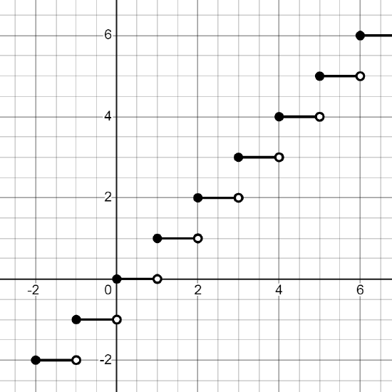
Now I ask myself what's happening in between? For \(x = 1.5\), the floor function will round down to 1 and spit that out. Same for \(x = 1.25, 1.75, 1.9999, ...\) and everything in between \(1\) and \(2\), BUT as soon as \(x = 2\), the function jumps up to the point \( (2,2)\) already plotted. I draw this on the graph like so:

The same phenomenon will happen between the other integers, hanging out as a flat line until it jumps to the next level. So the graph looks like this:
I recognize that going from \( f(x) = \lfloor x \rfloor \) to \( g(x) = \lfloor x \rfloor + 1 \) just took a vertical shift up by 1. So I just take every point on my graph and imagine sliding it directly upward by 1 unit. This allows me to sketch the graph of \( g \) below.

Sketch a graph of the absolute value function \( f(x) = |x| \), and use it to sketch the graph of \( g(x) = |x-2| \).
- Answer
-
Plot a few points and recognize the shape will use straight lines. The \(g\) is obtained from \(f\) by a horizontal shift to the right by 2. Your graphs should look like this (I don't care if you plot them both on the same plane like I did in the second image):

In studying transformations, we have technically been making functions out of other functions by performing additions, subtractions, and multiplications by scalars. Next, we're going to study how to make new functions from other functions by combining them in various ways!