8.8 Chapter 8 Study Guide

Definitions

• area: the measure of a two-dimensional region's interior space. Area quantities come with squared units like square feet, square miles, etc.
• perimeter: the sum of the lengths of all sides of a two-dimensional region. This comes with length units like inches, centimeters, etc.
• right triangles: triangles with one right interior angle. The sides on either side of the right angle are the legs and the other (longest) side is the hypotenuse.
• equilateral triangles: triangles with all sides equal. All interior angles are also equal, and must be \(60^\circ\).
• isosceles triangles: triangles with two equal sides. The angles opposite those two sides will also be equal.
• scalene triangles: triangles with sides of all different lengths.
• 45-45-90 triangles: special triangles whose angles are \(45^\circ, 45^\circ,\) and \(90^\circ\). The legs will be the same length, say \(x\), and the hypotenuse will be \(x\sqrt{2}\).
• 30-60-90 triangles: special triangles whose angles are \(30^\circ, 60^\circ,\) and \(90^\circ\). The shortest leg is opposite the smallest angle, and if that leg has length \(x\), then the other leg is \( x\sqrt{3}\) and the hypotenuse is \(2x\).
• Pythagorean triples: special right triangles whose side lengths are integers. The nicest ones are (3, 4, 5) and (5, 12, 13).
• rectangular prism: another word for box.
• similar triangles: triangles with all the same angles. Their corresponding side lengths are proportional!
• unit circle: a circle centered at the origin with radius 1, which we use to describe angles measured as counterclockwise rotation. Sweeping all the way around the circle travels from \(0\) to \(2\pi \) (\(0^\circ\) to \(360^\circ\)).
• degrees: units for the measure of an angle in which a full circle is \(360^\circ\).
• radians: units for the measure of an angle in which a full circle is \(2\pi\) radians.
• negative angles: angles measured in a clockwise direction instead of counterclockwise.
• coterminal angles: angles that "end up" in the exact same location on the unit circle. For example, \(90^\circ\) is \(\frac{\pi}{2}\), and so is \( \frac{5\pi}{2}\), it just loops all the way around the circle once before arriving there.
• quadrants: the four quarters of the 2D plane, divided up by the axes. Starting in the top right and moving counterclockwise, these are numbered I, II, III, and IV.
• reference angle: when you draw an angle in Quadrants II, III, or IV, the reference angle is the acute angle found by traveling directly to the horizontal axis.
  
• period: how long it takes for a trig function to complete a full cycle of its behavior. (How far you travel along the horizontal axis before it starts to repeat itself.)
• amplitude: the maximum distance sine or cosine travel away from the horizontal axis before turning around. For basic sine and cosine, this is 1.
• phase shift: a horizontal shift of the graph of sine or cosine.

Geometry Part

Essential 2D Formulas

• Rectangle with side lengths \(x\) and \(y\): area \(A = xy\), perimeter \(P = 2x+2y\).
• Square with side length \(x\): \(A = x^2\), \(P = 4x\).
• Triangle with base length \(b\) and height \(h\): \(A = \frac{1}{2}b h\). If a right triangle, the base and height are just the legs. To find perimeter, find all three side lengths and add.
• Circle with radius \(r\): \(A = \pi r^2\), perimeter is circumference \(C = 2\pi r\). To find the area of only part of a circle, just multiply by the proportion; for example, the area of a semicircle would be \(\frac{1}{2} \pi r^2\).

Essential 3D Formulas

• Rectangular Box with length \(x\), width \(y\), and height \(z\): volume \(V = xyz\), surface area \(S = 2xy + 2xz + 2yz\).
• Cube with side length \(x\): \(V = x^3\), \(S = 6x^2\).
• Cylinder with radius of base \(r\) and height \(h\): \(V = (\text{area of base})(\text{height}) = \pi r^2 h \), \(S = 2\pi r^2 + 2\pi r h\).
• Any extruded solid with consistent cross section, with area of the base \(A_b\) and height \(h\): \(V = A_b h\). To find surface area, decompose into the various sides as if you're cutting apart a cardboard shape, find their areas, and add.
• Sphere with radius \(r\): \(V = \frac{4}{3} \pi r^3\), \(S = 4\pi r^2\).
• (If needed) Right Circular Cone with radius of base \(r\) and height \(h\): \(V = \frac{1}{3} \pi r^2 h\).

Pythagorean Theorem

In a right triangle with leg lengths \(a\) and \(b\), and hypotenuse length \(c\), the following is true:

\[ a^2 + b^2 = c^2 \notag \]

This can be used to find the length of any side of a right triangle if you know the other two. Simply plug in the known values and solve for the third.

Attacking Problems Involving Geometry

Try...

1. Sketching a picture of the situation.
2. Labeling any known quantities, dimensions, etc.
3. Identifying what exactly you are trying to find for your answer.
4. Using geometric relationships between the different quantities to solve for your answer.

The Distance Formula

The distance between two points \( A: (x_1,y_1)\) and \(B: (x_2,y_2)\) is given by

\[ d(A,B) = \sqrt{ (x_2-x_1)^2 + (y_2-y_1)^2} \notag \]

Note: It doesn't matter which point you use as the "starting point," aka in what order you subtract the \(x\)-values and \(y\)-values, but you must be consistent in the choice. So you can't do \( (x_2-x_1)^2\) with \((y_1-y_2)^2\), you gotta keep the same order both times.

Similar Triangles

The corresponding sides of similar triangles are proportional. So if \(\Delta ABC \sim \Delta DEF \), we have

\[ \frac{AB}{DE} = \frac{BC}{EF} = \frac{AC}{DF} \notag \]

Trigonometry Part

Angles on the Unit Circle

Angle in Degrees	Angle in Radians	Angle on Circle
\(0^\circ\)	\(0\)
\(30^\circ\)	\( \dfrac{\pi}{6}\)
\(45^\circ\)	\( \dfrac{\pi}{4}\)
\(60^\circ\)	\( \dfrac{\pi}{3}\)
\(90^\circ\)	\( \dfrac{\pi}{2}\)
\(180^\circ\)	\( \pi\)
\(270^\circ\)	\( \dfrac{3\pi}{2}\)
\(360^\circ\)	\( 2\pi\)

To convert from degrees to radians, multiply the angle by \(\dfrac{\pi}{180}\) and simplify.

To convert from radians to degrees, multiply the angle by \( \dfrac{180}{\pi}\) and simplify.

The Trigonometric Ratios

The trigonometric ratios sine, cosine, tangent, cosecant, secant, and cotangent are defined as

\[ \sin \theta = \frac{opp}{hyp} \quad \quad \cos \theta = \frac{adj}{hyp} \quad \quad \tan \theta = \frac{opp}{adj} \notag \]

\[ \csc \theta = \frac{hyp}{opp} \quad \quad \sec \theta = \frac{hyp}{adj} \quad \quad \cot \theta = \frac{adj}{opp} \notag \]

Note: the ratios in the second row is simply the reciprocals of the ratios in the first row.

\[ \csc \theta = \frac{1}{\sin \theta} \quad \quad \sec \theta = \frac{1}{\cos \theta} \quad \quad \cot \theta = \frac{1}{\tan \theta} \notag \]

Also Note: \(\tan \theta = \dfrac{\sin \theta}{\cos\theta}\) and \( \cot \theta = \dfrac{\cos \theta}{\sin \theta}\)! This is very important. Confirm by dividing the side ratios of sine and cosine to see that they turn out to be \(\frac{opp}{adj}\), etc.

Memory Trick: You can memorize these ratios with the "SOH-CAH-TOA" mnemonic, which stands for "Sine:Opposite/Hypotenuse, Cosine:Adjacent/Hypotenuse, Tangent:Opposite/Adjacent."

Using One Trig Ratio to Find the Others

You will be given a value like \( \sin \theta = \frac{a}{b}\) and information about which quadrant the angle lies in. The quadrants of the plane are shown below:

1. Sketch a right triangle in the plane in the appropriate quadrant and label \(\theta\). Label two of the sides \(a\) and \(b\), according to the trig ratio given.
2. Use the Pythagorean Theorem to find the third side of the triangle.
3. Use the triangle to find the other trig ratios as usual.

Example: for the given "\( \sin \theta = \frac{7}{25}\) and \(\theta\) is in Quadrant II," you would sketch this triangle:

Then use the Pythagorean Theorem to complete the triangle and find all the trig ratios by definition.

Values of Sine and Cosine From Unit Circle

Graphs of Trig Functions

Graph	Observations
	Periodic behavior: The function starts at \((0,0)\), does a hill, does a valley, and returns to the height of 0 by \(x = 2\pi\)...and then it repeats the same pattern. This is called being periodic with period \(2\pi\), because it takes from 0 to \(2\pi\) to do one full cycle. The points called out on the graph are the easiest ones to find on the unit circle, the cardinal points. Sine passes through \( (0,0)\). That is, \(\sin(0) = 0\). He is not symmetric about the \(y\)-axis. The function values are bounded between \(-1\) and \(1\). Aka, the function never goes higher than \(1\) or lower than \(-1\). Sine is nice and smooth and continuous, meaning you can draw him without ever having to pick up your pencil. The function is defined for negative values of \(x\): these are just negative angles, which were discussed in the last section and its exercises. In fact, his domain is all real numbers.
	Periodic behavior: Cosine also repeats his behavior, starting the cycle over every time you travel a distance of \(2\pi\). You can see he starts at a height of \(1\) at \(x = 0\), performs a full down-and-up cycle, and comes back to a height of \(1\) at \(x = 2\pi\). The points labeled are again the easiest ones to find from the unit circle. You can compare them to confirm. Cosine passes through \( (0,1)\). That is, \(\cos(0) = 1\). He is symmetric about the \(y\)-axis. His \(y\)-value heights are also trapped between \(-1\) and \(1\). Cosine is also nice and smooth and continuous, with domain all real numbers again.
	Periodic behavior: Tangent repeats himself, but his period is only \(\pi\). Vertical asymptotes: Tangent is undefined at any \(x\)-value that is an odd multiple of \(\pi/2\). This is because at those locations, \(\cos x\) is zero, and you can't compute \(\tan x = \frac{ \sin x}{\cos x}\)! You see vertical axymptotes at those locations, and tangent hugs them but never touches them. This means tangent is not continuous because you have to keep picking up your pencil to hop over those asymptotes! The locations where tangent is \(1\) are \(\pi/4\) and \(5\pi/4\). These are the "quarters" locations in Quadrants I and III, and these are the locations where sine and cosine have the same value. Thus when you divide them to find tangent, you get \(1\). Tangent passes through \( (0,0)\), and passes through the \(x\)-axis at every multiple of \(\pi\). In math symbols, you can write "\(\tan x = 0\) whenever \(x = nx\) for some integer \(n\)." Due to those undefined values, the domain of tangent is all real numbers except odd multiples of \( \pi/2\). You can write this in math as "\(x \neq (2k-1)\frac{\pi}{2}\) for \(k\) any integer." Try some options for \(k\) to see that this expression will give you odd multiples like \( -\frac{\pi}{2}, \frac{3\pi}{2}, \frac{5\pi}{2}\), etc.

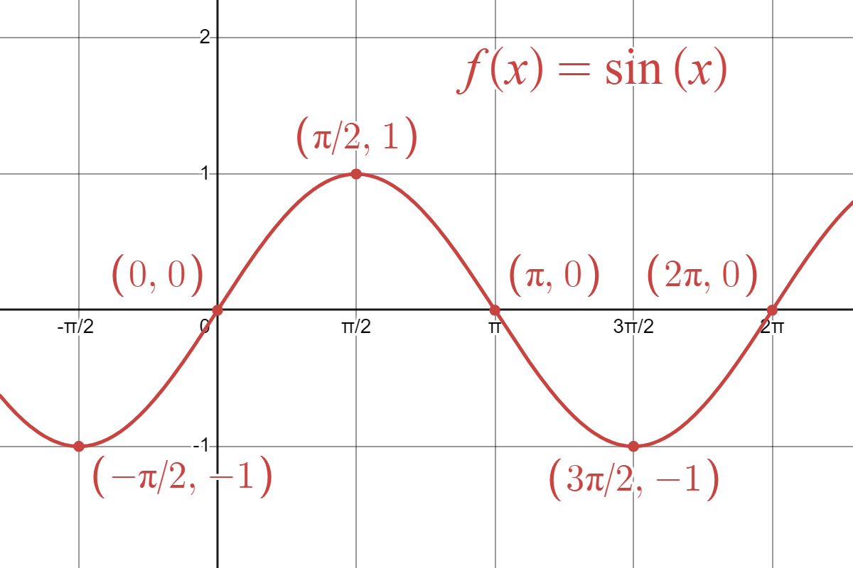
To sketch the graph of sine or cosine,

1. Sketch a baby unit circle in the margin and label the cardinal points \( (1,0), (0,1), (-1,0),\) and \( (0,-1)\). These give you the values of sine and cosine at the inputs \(0, \frac{\pi}{2}, \pi, \frac{3\pi}{2},\) respectively.
2. Draw the axes for your function's graph and mark those same angles on the horizontal axis. Then use your unit circle to plot the function's points at those values.
3. Use your knowledge of symmetry and the hilly shape of sine/cosine to smoothly connect the dots and follow the pattern to repeat periodically.

To sketch the graph of tangent,

1. Sketch the \(x\)- and \(y\)-axes and mark the \(x\)-values \(\frac{\pi}{4}, \frac{\pi}{2}, \frac{3\pi}{4}, \pi, \frac{5\pi}{4}, \frac{3\pi}{2}, ...\) etc.
2. Recall the locations where tangent is \(0\) (anywhere that sine is 0): at \(..., -\pi, 0, \pi, 2\pi, 3\pi, ...\) etc. At those locations, the function crosses the \(x\)-axis, so plot those roots.
3. Recall the locations where tangent is \(1\): at \(\frac{\pi}{4}\) and \(\frac{5\pi}{4}\), as discussed above. Plot those points, \( (\pi/4, 1)\) and \(5\pi/4\).
4. Recall the locations where tangent is \(-1\): at \(-\frac{\pi}{4}\) and \(\frac{3\pi}{4}\), etc. Plot those points too.
5. Sketch in the vertical asymptotes: dotted vertical lines passing through \(\frac{\pi}{2}, \frac{3\pi}{2}, \) etc. on the \(x\)-axis.
6. Use your knowledge of the shape of tangent to smoothly connect the dots and follow the asymptotes up and down. Repeat the behavior periodically.

Graphs of the three reciprocal trig functions:

Transformed Trig Functions

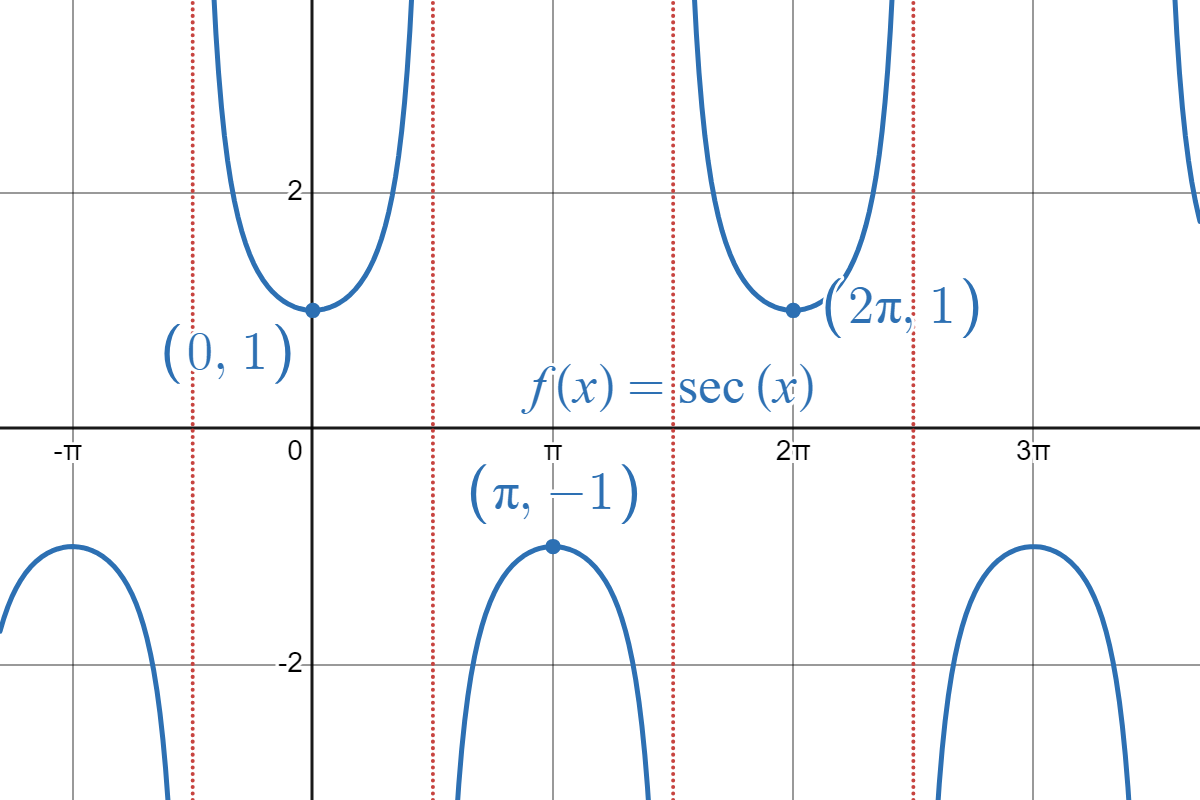For a function of the form \(f(x) = a \sin (x + c) \) or \(a \cos (x + c)\),

• \(|a|\) is the amplitude
• \(c\) gives the phase shift (to the left if \(+\), to the right if \(-\))
• the period is \(2\pi\)

For a function of the form \( f(x) = a \sin (bx) \) or \(a \cos (bx)\),

• \(|a|\) is the amplitude
• \(b\) causes a horizontal shrink if \(b>1\), and a horizontal stretch if \(0<b<1\)
• the period is \( \frac{2\pi}{b}\)

To sketch the graph of a transformed trig function,

1. sketch the OG trig function first with its important signpost points
2. determine the transformations that have occurred and how they change the signpost points
3. plot the new signpost points and smoothly connect the dots

Inverse Trig Functions

Function	Observations
	Domain: arcsine only takes inputs \( -1 \leq x \leq 1\), because those are the only outputs of sine. In interval notation, \( [-1, 1]\). Range: arcsine only outputs values from\( \frac{-\pi}{2}\) to \( \frac{\pi}{2} \), because that was the restricted domain we chose for sine. You can think of those angles as the "right half" of the unit circle. In interval notation, \( [-\pi/2, \pi/2]\). Arcsine passes through \( (0,0)\) because \( \sin(\textcolor{red}{0}) = \textcolor{blue}{0}\), so we must have \( \arcsin(\textcolor{blue}{0}) = \textcolor{red}{0} \). Similarly, it has signpost endpoints \( (-1, -\pi/2)\) and \( (1, \pi/2) \).
	Domain: arccosine takes inputs \( -1 \leq x \leq 1\) for the same reasons as arcsine. In interval notation, \( [-1, 1]\). Range: arccosine only spits out values from \( 0\) to \( \pi\), because that's the restricted domain we use for cosine (by tradition). You can remember those angles as the "top half" of the unit circle. In interval notation, \( [0, \pi]\). Arccosine's signpost points are the endpoints \( (-1,\pi)\) and \( (1,0) \), and the \(y\)-intercept \( (0, \pi/2) \).
	Domain: Arctangent takes all real numbers as inputs, because that's the range of tangent (he goes up forever and down forever). In interval notation, \( [-\infty, \infty]\). Range: Arctangent spits out values strictly between \( -\pi/2\) and \( \pi/2 \), because that's the conventional restricted domain of tangent. In interval notation, \( (-\pi/2, \pi/2)\). Going off to the right forever, arctangent approaches the horizontal asymptote \( y = \pi/2\) from below. Going off to the left, it approaches \(y = - \pi/2\) from above. When sketching arctangent, you should plot the easy points \( (0,0), (-1, -\pi/4),\) and \( (1, \pi/4) \), drop in your horizontal asymptotes, and then smoothly swoop in through the points.

There are inverse functions for the reciprocal trig functions:

• arccosecant (\( \operatorname{arccsc} x\)): domain \( (-\infty, -1] \cup [1, \infty) \) and range \([-\pi/2, \pi/2]\) (this is also the restricted domain for cosecant)
• arcsecant (\( \operatorname{arcsec} x\)): domain \( (-\infty, -1] \cup [1, \infty) \) and range \([0, \pi]\) (this is also the restricted domain for secant)
• arccotangent (\(\operatorname{arccot} x\)): domain \( (-\infty, \infty)\) and range \( (0,\pi) \) (this is also the restricted domain for cotangent)

To evaluate an inverse trig function,

1. Translate it to an equation involving the regular trig function. For example, "\( \arcsin (1) = ?\)" translates to "\( \sin(?) = 1\)."
2. Recall your unit circle to figure out which angles give you the desired outcome.
3. Report the angle that falls in the allowable range of the inverse trig function.

The Pythagorean Identities

For any consistent expression \(A\), we have

\[ \sin^2 A + \cos^2 A = 1. \notag \]

(Notation note: recall that \( \sin^2 A \) just means \( (\sin A)^2\).)

We also have

\[ \tan^2 A + 1 = \sec^2 A, \quad \quad 1 + \cot^2 A = \csc^2 A \notag \]

Even/Odd Identities

Since sine is an odd function and cosine is an even function,

\[ \sin(-x) = - \sin x \quad \text{ and } \quad \cos(-x) = \cos x \notag \]

Sum/Difference Formulas

For sine, the formulas for addition or subtraction in the input have mixed terms:

\[ \sin(A \textcolor{red}{+}B) = \sin A \cos B \textcolor{red}{+} \cos A \sin B \quad \quad \sin(A \textcolor{red}{-}B) = \sin A \cos B \textcolor{red}{-} \cos A \sin B \notag \]

For cosine, we have matching terms:

\[ \cos( A \textcolor{red}{+} B) = \cos A \cos B \textcolor{red}{-} \sin A \sin B \quad \quad \cos (A \textcolor{red}{-} B) = \cos A \cos B \textcolor{red}{+} \sin A \sin B \notag \]

Also, for tangent, if needed, we have:

\[ \tan(A + B) = \frac{ \tan A + \tan B}{1- \tan A \tan B} \quad \quad \tan(A-B) = \frac{ \tan A - \tan B}{1 + \tan A \tan B} \notag \]

Double Angle Formulas

For sine, we have

\[ \sin 2A = 2 \sin A \cos A \notag \]

For cosine, we have several equivalent expressions

\[ \cos 2A = \textcolor{red}{\cos^2 A - \sin^2 A} = \textcolor{blue}{ 1 - 2 \sin^2 A} = \textcolor{green}{2 \cos^2 A - 1} \notag \]

Also, if needed, we have for tangent

\[ \tan 2A = \frac{2 \tan A}{1 - \tan^2 x} \notag \]

Solving Trig Equations

To find all solutions to a trigonometric equation,

1. Use algebra to manipulate the equation until it consists of one single trig function isolated on one side of the equals.
2. Find all the solutions in the usual unit circle (angles between \(0\) and \(2\pi\)).
3. List all solutions by adding integer multiples of the period to the solutions.

Algebra tricks and techniques to try:

• Translate everything into sines and cosines and simplify.
• If there are multiple fraction terms, find a common denominator.
• On the other hand, if there is a fraction with multiple terms added/subtracted in the numerator, try splitting it into multiple fractions in case anything will simplify.
• Bring everything to one side and then try factoring and splitting into cases.
• If there are absolute value bars, split into two cases.
• Try squaring both sides to see if it makes it easier, but you must check your answers at the end to make sure they work in the original equation!
• Look for expressions that look like double-angle or sum/difference formulas in case you can replace them with something simpler.
• Try getting all the trig to be in terms of a single type (like using the Pythagorean Identity to replace \( \sin^2 x\) with \( 1- \cos^2 x\)).
• If there is a complicated input, first ignore it (you could replace it with a nickname variable) to find the angles you want, and then adjust as necessary.
• When in doubt, just rewrite the equation in many different ways using identities to replace/condense/expand/simplify/manipulate the various parts, until something works! "Write down true things."