
3.9E: Exercises for Section 3.9
- Page ID
- 149890
\( \newcommand{\vecs}[1]{\overset { \scriptstyle \rightharpoonup} {\mathbf{#1}} } \)
\( \newcommand{\vecd}[1]{\overset{-\!-\!\rightharpoonup}{\vphantom{a}\smash {#1}}} \)
\( \newcommand{\id}{\mathrm{id}}\) \( \newcommand{\Span}{\mathrm{span}}\)
( \newcommand{\kernel}{\mathrm{null}\,}\) \( \newcommand{\range}{\mathrm{range}\,}\)
\( \newcommand{\RealPart}{\mathrm{Re}}\) \( \newcommand{\ImaginaryPart}{\mathrm{Im}}\)
\( \newcommand{\Argument}{\mathrm{Arg}}\) \( \newcommand{\norm}[1]{\| #1 \|}\)
\( \newcommand{\inner}[2]{\langle #1, #2 \rangle}\)
\( \newcommand{\Span}{\mathrm{span}}\)
\( \newcommand{\id}{\mathrm{id}}\)
\( \newcommand{\Span}{\mathrm{span}}\)
\( \newcommand{\kernel}{\mathrm{null}\,}\)
\( \newcommand{\range}{\mathrm{range}\,}\)
\( \newcommand{\RealPart}{\mathrm{Re}}\)
\( \newcommand{\ImaginaryPart}{\mathrm{Im}}\)
\( \newcommand{\Argument}{\mathrm{Arg}}\)
\( \newcommand{\norm}[1]{\| #1 \|}\)
\( \newcommand{\inner}[2]{\langle #1, #2 \rangle}\)
\( \newcommand{\Span}{\mathrm{span}}\) \( \newcommand{\AA}{\unicode[.8,0]{x212B}}\)
\( \newcommand{\vectorA}[1]{\vec{#1}} % arrow\)
\( \newcommand{\vectorAt}[1]{\vec{\text{#1}}} % arrow\)
\( \newcommand{\vectorB}[1]{\overset { \scriptstyle \rightharpoonup} {\mathbf{#1}} } \)
\( \newcommand{\vectorC}[1]{\textbf{#1}} \)
\( \newcommand{\vectorD}[1]{\overrightarrow{#1}} \)
\( \newcommand{\vectorDt}[1]{\overrightarrow{\text{#1}}} \)
\( \newcommand{\vectE}[1]{\overset{-\!-\!\rightharpoonup}{\vphantom{a}\smash{\mathbf {#1}}}} \)
\( \newcommand{\vecs}[1]{\overset { \scriptstyle \rightharpoonup} {\mathbf{#1}} } \)
\( \newcommand{\vecd}[1]{\overset{-\!-\!\rightharpoonup}{\vphantom{a}\smash {#1}}} \)
\(\newcommand{\avec}{\mathbf a}\) \(\newcommand{\bvec}{\mathbf b}\) \(\newcommand{\cvec}{\mathbf c}\) \(\newcommand{\dvec}{\mathbf d}\) \(\newcommand{\dtil}{\widetilde{\mathbf d}}\) \(\newcommand{\evec}{\mathbf e}\) \(\newcommand{\fvec}{\mathbf f}\) \(\newcommand{\nvec}{\mathbf n}\) \(\newcommand{\pvec}{\mathbf p}\) \(\newcommand{\qvec}{\mathbf q}\) \(\newcommand{\svec}{\mathbf s}\) \(\newcommand{\tvec}{\mathbf t}\) \(\newcommand{\uvec}{\mathbf u}\) \(\newcommand{\vvec}{\mathbf v}\) \(\newcommand{\wvec}{\mathbf w}\) \(\newcommand{\xvec}{\mathbf x}\) \(\newcommand{\yvec}{\mathbf y}\) \(\newcommand{\zvec}{\mathbf z}\) \(\newcommand{\rvec}{\mathbf r}\) \(\newcommand{\mvec}{\mathbf m}\) \(\newcommand{\zerovec}{\mathbf 0}\) \(\newcommand{\onevec}{\mathbf 1}\) \(\newcommand{\real}{\mathbb R}\) \(\newcommand{\twovec}[2]{\left[\begin{array}{r}#1 \\ #2 \end{array}\right]}\) \(\newcommand{\ctwovec}[2]{\left[\begin{array}{c}#1 \\ #2 \end{array}\right]}\) \(\newcommand{\threevec}[3]{\left[\begin{array}{r}#1 \\ #2 \\ #3 \end{array}\right]}\) \(\newcommand{\cthreevec}[3]{\left[\begin{array}{c}#1 \\ #2 \\ #3 \end{array}\right]}\) \(\newcommand{\fourvec}[4]{\left[\begin{array}{r}#1 \\ #2 \\ #3 \\ #4 \end{array}\right]}\) \(\newcommand{\cfourvec}[4]{\left[\begin{array}{c}#1 \\ #2 \\ #3 \\ #4 \end{array}\right]}\) \(\newcommand{\fivevec}[5]{\left[\begin{array}{r}#1 \\ #2 \\ #3 \\ #4 \\ #5 \\ \end{array}\right]}\) \(\newcommand{\cfivevec}[5]{\left[\begin{array}{c}#1 \\ #2 \\ #3 \\ #4 \\ #5 \\ \end{array}\right]}\) \(\newcommand{\mattwo}[4]{\left[\begin{array}{rr}#1 \amp #2 \\ #3 \amp #4 \\ \end{array}\right]}\) \(\newcommand{\laspan}[1]{\text{Span}\{#1\}}\) \(\newcommand{\bcal}{\cal B}\) \(\newcommand{\ccal}{\cal C}\) \(\newcommand{\scal}{\cal S}\) \(\newcommand{\wcal}{\cal W}\) \(\newcommand{\ecal}{\cal E}\) \(\newcommand{\coords}[2]{\left\{#1\right\}_{#2}}\) \(\newcommand{\gray}[1]{\color{gray}{#1}}\) \(\newcommand{\lgray}[1]{\color{lightgray}{#1}}\) \(\newcommand{\rank}{\operatorname{rank}}\) \(\newcommand{\row}{\text{Row}}\) \(\newcommand{\col}{\text{Col}}\) \(\renewcommand{\row}{\text{Row}}\) \(\newcommand{\nul}{\text{Nul}}\) \(\newcommand{\var}{\text{Var}}\) \(\newcommand{\corr}{\text{corr}}\) \(\newcommand{\len}[1]{\left|#1\right|}\) \(\newcommand{\bbar}{\overline{\bvec}}\) \(\newcommand{\bhat}{\widehat{\bvec}}\) \(\newcommand{\bperp}{\bvec^\perp}\) \(\newcommand{\xhat}{\widehat{\xvec}}\) \(\newcommand{\vhat}{\widehat{\vvec}}\) \(\newcommand{\uhat}{\widehat{\uvec}}\) \(\newcommand{\what}{\widehat{\wvec}}\) \(\newcommand{\Sighat}{\widehat{\Sigma}}\) \(\newcommand{\lt}{<}\) \(\newcommand{\gt}{>}\) \(\newcommand{\amp}{&}\) \(\definecolor{fillinmathshade}{gray}{0.9}\)For exercises 1 - 5, examine the graphs. Identify where the vertical asymptotes are located.
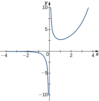
1)
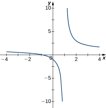
- Answer
- \(x=1\)
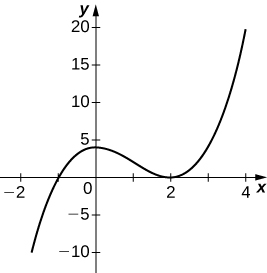
2)
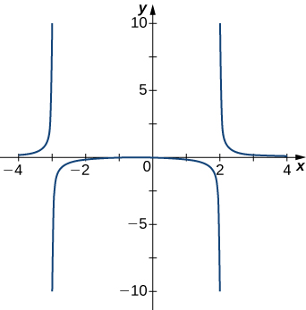
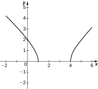
3)
- Answer
- \(x=−1,\;x=2\)
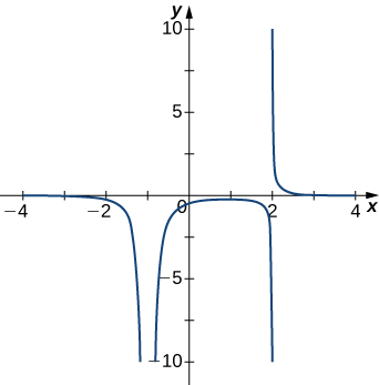
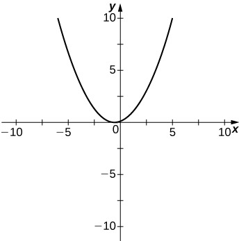
4)
5)
- Answer
- \(x=0\)
For the functions \(f(x)\) in exercises 6 - 10, determine whether there is an asymptote at \(x=a\). Justify your answer without graphing on a calculator.
6) \(f(x)=\dfrac{x+1}{x^2+5x+4},\quad a=−1\)
7) \(f(x)=\dfrac{x}{x−2},\quad a=2\)
- Answer
- Yes, there is a vertical asymptote at \(x = 2\).
8) \(f(x)=(x+2)^{3/2},\quad a=−2\)
9) \(f(x)=(x−1)^{−1/3},\quad a=1\)
- Answer
- Yes, there is vertical asymptote at \(x = 1\).
10) \(f(x)=1+x^{−2/5},\quad a=1\)
In exercises 11 - 20, evaluate the limit.
11) \(\displaystyle \lim_{x→∞}\frac{1}{3x+6}\)
- Answer
- \(\displaystyle \lim_{x→∞}\frac{1}{3x+6} = 0\)
12) \(\displaystyle \lim_{x→∞}\frac{2x−5}{4x}\)
13) \(\displaystyle \lim_{x→∞}\frac{x^2−2x+5}{x+2}\)
- Answer
- \(\displaystyle \lim_{x→∞}\frac{x^2−2x+5}{x+2} = ∞\)
14) \(\displaystyle \lim_{x→−∞}\frac{3x^3−2x}{x^2+2x+8}\)
15) \(\displaystyle \lim_{x→−∞}\frac{x^4−4x^3+1}{2−2x^2−7x^4}\)
- Answer
- \(\displaystyle \lim_{x→−∞}\frac{x^4−4x^3+1}{2−2x^2−7x^4} = −\frac{1}{7}\)
16) \(\displaystyle \lim_{x→∞}\frac{3x}{\sqrt{x^2+1}}\)
17) \(\displaystyle \lim_{x→−∞}\frac{\sqrt{4x^2−1}}{x+2}\)
- Answer
- \(\displaystyle \lim_{x→−∞}\frac{\sqrt{4x^2−1}}{x+2} = -2\)
18) \(\displaystyle \lim_{x→∞}\frac{4x}{\sqrt{x^2−1}}\)
19) \(\displaystyle \lim_{x→−∞}\frac{4x}{\sqrt{x^2−1}}\)
- Answer
- \(\displaystyle \lim_{x→−∞}\frac{4x}{\sqrt{x^2−1}} = -4\)
20) \(\displaystyle \lim_{x→∞}\frac{2\sqrt{x}}{x−\sqrt{x}+1}\)
For exercises 21 - 29, find the horizontal and vertical asymptotes.
21) \(f(x)=x−\dfrac{9}{x}\)
- Answer
- Horizontal: none,
Vertical: \(x=0\)
22) \(f(x)=\dfrac{1}{1−x^2}\)
23) \(f(x)=\dfrac{x^3}{4−x^2}\)
- Answer
- Horizontal: none,
Vertical: \(x=±2\)
24) \(f(x)=\dfrac{x^2+3}{x^2+1}\)
25) \(f(x)=\dfrac{3x^2-3x}{x^2+x-12}\)
- Answer
- Horizontal: \(y=3\)
Vertical: \(x=-4,x=3\)
26) \(f(x)=\dfrac{1}{x^3+x^2}\)
- Answer
- Horizontal: \(y=0,\)
Vertical: \(x=0\) and \(x=−1\)
27) \(f(x)=\dfrac{1}{x−1}−2x\)
28) \(f(x)=\dfrac{x^3+1}{x^3−1}\)
- Answer
- Horizontal: \(y=1,\)
Vertical: \(x=1\)
29) \(f(x)=\dfrac{1}{x}−\sqrt{x}\)
For exercises 30-33, construct a function \(f(x)\) that has the given asymptotes.
30) \(x=1\) and \(y=2\)
- Answer
- Answers will vary, for example: \(y=\dfrac{2x}{x−1}\)
31) \(x=1\) and \(y=0\)
32) \(y=4, \;x=−1\)
- Answer
- Answers will vary, for example: \(y=\dfrac{4x}{x+1}\)
33) \(x=0\)
In exercises 34-38 graph the function on a graphing calculator on the window \(x=[−5,5]\) and estimate the horizontal asymptote or limit. Then, calculate the actual horizontal asymptote or limit.
34) [T] \(f(x)=\dfrac{1}{x+10}\)
- Answer
- \(\displaystyle \lim_{x→∞}\frac{1}{x+10}=0\) so \(f\) has a horizontal asymptote of \(y=0\).
35) [T] \(f(x)=\dfrac{x+1}{x^2+7x+6}\)
36) [T] \(\displaystyle \lim_{x→−∞}x^2+10x+25\)
- Answer
- \(\displaystyle \lim_{x→−∞}x^2+10x+25 = ∞\)
37) [T] \(\displaystyle \lim_{x→−∞}\frac{x+2}{x^2+7x+6}\)
38) [T] \(\displaystyle \lim_{x→∞}\frac{3x+2}{x+5}\)
- Answer
- \(\displaystyle \lim_{x→∞}\frac{3x+2}{x+5}=3\) so this function has a horizontal asymptote of \(y=3\).
In exercises 39-47, draw a graph of the functions without using a calculator. Be sure to notice all important features of the graph: local maxima and minima, inflection points, and asymptotic behavior.
39) \(y=3x^2+2x+4\)
40) \(y=x^3−3x^2+4\)
- Answer
41) \(y=\dfrac{2x+1}{x^2+6x+5}\)
42) \(y=\dfrac{2x+2}{x-1}\)
- Answer
43) \(y=\dfrac{x^3+4x^2+3x}{3x+9}\)
- Answer
44) \(y=\dfrac{x^2+x−2}{x^2−3x−4}\)
45) \(y=\sqrt{x^2−5x+4}\)
- Answer
46) \(y=e^x−x^3\)
47) \(y=x\ln(x), \quad x>0\)
48) For \(f(x)=\dfrac{P(x)}{Q(x)}\) to have an asymptote at \(y=2\) then the polynomials \(P(x)\) and \(Q(x)\) must have what relation?
49) For \(f(x)=\dfrac{P(x)}{Q(x)}\) to have an asymptote at \(x=0\), then the polynomials \(P(x)\) and \(Q(x).\) must have what relation?
- Answer
- \(Q(x).\) must have have \(x^{k+1}\) as a factor, where \(P(x)\) has \(x^k\) as a factor.
50) If \(f′(x)\) has asymptotes at \(y=3\) and \(x=1\), then \(f(x)\) has what asymptotes?
51) Both \(f(x)=\dfrac{1}{x−1}\) and \(g(x)=\dfrac{1}{(x−1)^2}\) have asymptotes at \(x=1\) and \(y=0.\) What is the most obvious difference between these two functions?
- Answer
- \(\displaystyle \lim_{x→1^−}f(x)=-\infty \text{ and } \lim_{x→1^−}g(x)=\infty\)
52) True or false: Every ratio of polynomials has vertical asymptotes.