
4.1: Exponential Functions
- Page ID
- 130967

\( \newcommand{\vecs}[1]{\overset { \scriptstyle \rightharpoonup} {\mathbf{#1}} } \)
\( \newcommand{\vecd}[1]{\overset{-\!-\!\rightharpoonup}{\vphantom{a}\smash {#1}}} \)
\( \newcommand{\dsum}{\displaystyle\sum\limits} \)
\( \newcommand{\dint}{\displaystyle\int\limits} \)
\( \newcommand{\dlim}{\displaystyle\lim\limits} \)
\( \newcommand{\id}{\mathrm{id}}\) \( \newcommand{\Span}{\mathrm{span}}\)
( \newcommand{\kernel}{\mathrm{null}\,}\) \( \newcommand{\range}{\mathrm{range}\,}\)
\( \newcommand{\RealPart}{\mathrm{Re}}\) \( \newcommand{\ImaginaryPart}{\mathrm{Im}}\)
\( \newcommand{\Argument}{\mathrm{Arg}}\) \( \newcommand{\norm}[1]{\| #1 \|}\)
\( \newcommand{\inner}[2]{\langle #1, #2 \rangle}\)
\( \newcommand{\Span}{\mathrm{span}}\)
\( \newcommand{\id}{\mathrm{id}}\)
\( \newcommand{\Span}{\mathrm{span}}\)
\( \newcommand{\kernel}{\mathrm{null}\,}\)
\( \newcommand{\range}{\mathrm{range}\,}\)
\( \newcommand{\RealPart}{\mathrm{Re}}\)
\( \newcommand{\ImaginaryPart}{\mathrm{Im}}\)
\( \newcommand{\Argument}{\mathrm{Arg}}\)
\( \newcommand{\norm}[1]{\| #1 \|}\)
\( \newcommand{\inner}[2]{\langle #1, #2 \rangle}\)
\( \newcommand{\Span}{\mathrm{span}}\) \( \newcommand{\AA}{\unicode[.8,0]{x212B}}\)
\( \newcommand{\vectorA}[1]{\vec{#1}} % arrow\)
\( \newcommand{\vectorAt}[1]{\vec{\text{#1}}} % arrow\)
\( \newcommand{\vectorB}[1]{\overset { \scriptstyle \rightharpoonup} {\mathbf{#1}} } \)
\( \newcommand{\vectorC}[1]{\textbf{#1}} \)
\( \newcommand{\vectorD}[1]{\overrightarrow{#1}} \)
\( \newcommand{\vectorDt}[1]{\overrightarrow{\text{#1}}} \)
\( \newcommand{\vectE}[1]{\overset{-\!-\!\rightharpoonup}{\vphantom{a}\smash{\mathbf {#1}}}} \)
\( \newcommand{\vecs}[1]{\overset { \scriptstyle \rightharpoonup} {\mathbf{#1}} } \)
\(\newcommand{\longvect}{\overrightarrow}\)
\( \newcommand{\vecd}[1]{\overset{-\!-\!\rightharpoonup}{\vphantom{a}\smash {#1}}} \)
\(\newcommand{\avec}{\mathbf a}\) \(\newcommand{\bvec}{\mathbf b}\) \(\newcommand{\cvec}{\mathbf c}\) \(\newcommand{\dvec}{\mathbf d}\) \(\newcommand{\dtil}{\widetilde{\mathbf d}}\) \(\newcommand{\evec}{\mathbf e}\) \(\newcommand{\fvec}{\mathbf f}\) \(\newcommand{\nvec}{\mathbf n}\) \(\newcommand{\pvec}{\mathbf p}\) \(\newcommand{\qvec}{\mathbf q}\) \(\newcommand{\svec}{\mathbf s}\) \(\newcommand{\tvec}{\mathbf t}\) \(\newcommand{\uvec}{\mathbf u}\) \(\newcommand{\vvec}{\mathbf v}\) \(\newcommand{\wvec}{\mathbf w}\) \(\newcommand{\xvec}{\mathbf x}\) \(\newcommand{\yvec}{\mathbf y}\) \(\newcommand{\zvec}{\mathbf z}\) \(\newcommand{\rvec}{\mathbf r}\) \(\newcommand{\mvec}{\mathbf m}\) \(\newcommand{\zerovec}{\mathbf 0}\) \(\newcommand{\onevec}{\mathbf 1}\) \(\newcommand{\real}{\mathbb R}\) \(\newcommand{\twovec}[2]{\left[\begin{array}{r}#1 \\ #2 \end{array}\right]}\) \(\newcommand{\ctwovec}[2]{\left[\begin{array}{c}#1 \\ #2 \end{array}\right]}\) \(\newcommand{\threevec}[3]{\left[\begin{array}{r}#1 \\ #2 \\ #3 \end{array}\right]}\) \(\newcommand{\cthreevec}[3]{\left[\begin{array}{c}#1 \\ #2 \\ #3 \end{array}\right]}\) \(\newcommand{\fourvec}[4]{\left[\begin{array}{r}#1 \\ #2 \\ #3 \\ #4 \end{array}\right]}\) \(\newcommand{\cfourvec}[4]{\left[\begin{array}{c}#1 \\ #2 \\ #3 \\ #4 \end{array}\right]}\) \(\newcommand{\fivevec}[5]{\left[\begin{array}{r}#1 \\ #2 \\ #3 \\ #4 \\ #5 \\ \end{array}\right]}\) \(\newcommand{\cfivevec}[5]{\left[\begin{array}{c}#1 \\ #2 \\ #3 \\ #4 \\ #5 \\ \end{array}\right]}\) \(\newcommand{\mattwo}[4]{\left[\begin{array}{rr}#1 \amp #2 \\ #3 \amp #4 \\ \end{array}\right]}\) \(\newcommand{\laspan}[1]{\text{Span}\{#1\}}\) \(\newcommand{\bcal}{\cal B}\) \(\newcommand{\ccal}{\cal C}\) \(\newcommand{\scal}{\cal S}\) \(\newcommand{\wcal}{\cal W}\) \(\newcommand{\ecal}{\cal E}\) \(\newcommand{\coords}[2]{\left\{#1\right\}_{#2}}\) \(\newcommand{\gray}[1]{\color{gray}{#1}}\) \(\newcommand{\lgray}[1]{\color{lightgray}{#1}}\) \(\newcommand{\rank}{\operatorname{rank}}\) \(\newcommand{\row}{\text{Row}}\) \(\newcommand{\col}{\text{Col}}\) \(\renewcommand{\row}{\text{Row}}\) \(\newcommand{\nul}{\text{Nul}}\) \(\newcommand{\var}{\text{Var}}\) \(\newcommand{\corr}{\text{corr}}\) \(\newcommand{\len}[1]{\left|#1\right|}\) \(\newcommand{\bbar}{\overline{\bvec}}\) \(\newcommand{\bhat}{\widehat{\bvec}}\) \(\newcommand{\bperp}{\bvec^\perp}\) \(\newcommand{\xhat}{\widehat{\xvec}}\) \(\newcommand{\vhat}{\widehat{\vvec}}\) \(\newcommand{\uhat}{\widehat{\uvec}}\) \(\newcommand{\what}{\widehat{\wvec}}\) \(\newcommand{\Sighat}{\widehat{\Sigma}}\) \(\newcommand{\lt}{<}\) \(\newcommand{\gt}{>}\) \(\newcommand{\amp}{&}\) \(\definecolor{fillinmathshade}{gray}{0.9}\)In this section, we will study a different family of functions, and investigate their role in financial mathematics.
- Recognize examples and non-examples of exponential functions
- Distinguish between exponential growth and exponential decay using context clues and algebra
- Identify initial values and growth rates in context and use them to write exponential functions
Exponential Functions: Basic Intuition and Definition
We will start this section with a hands-on exercise. You are encouraged to actually complete the task before moving on for maximum impact.
Find a regular piece of paper (lined paper, printer paper, used scratch paper are all fine -- but you want approximately \(8.5\) inches by \(11\) inches in size). This paper is about \(0.1\) millimeters thick. Your goal will be to describe the thickness of the stack of paper as you fold it in half multiple times.
To get you started: after 0 folds, the stack of paper is \(0.1\) millimeters thick since there is only one piece of paper in the stack. Now fold the paper in half. Then there are two sheets of paper in the stack, so the entire stack is \(0.2\) millimeters thick.
Now fold it in half again, but perpendicular to your first fold. Your paper should look like this:

There are four sheets of paper in this stack, meaning that if you were to draw a line through the center of the stack from top to bottom, you would intersect the paper four times. The thickness of this stack is 0.4 millimeters.
| Number of folds | Number of sheets | Thickness (in millimeters) |
| 0 | 1 | 0.1 |
| 1 | 2 | 0.2 |
| 2 | 4 | 0.4 |
| 3 | ||
| 4 | ||
| 5 | ||
| 6 | ||
| 7 |
Here are some questions to think about:
- Can you find a function that describes the thickness of the stack based on the number of folds?
- How many folds would it take for the stack of paper to reach the moon? (Pretend your paper is large enough to keep folding it as many times as you need.)
In the previous exercise, you may have noticed several patterns in your table, even if you were not able write a function that described the situation. This is a difficult question because the behavior above is not described by a linear function, which is the only type of function we've studied in detail. Instead, it is a new type of function, called an exponential function.
An exponential function is a function that can be written \(f(x) = a(1+r)^x\) for some numbers \(a\) and \(r\). The number \(r\) is called the growth rate or decay rate of the function, and represents the percent change of the function as a decimal. If \(r\) is positive, it is a growth rate, and if \(r\) is negative, it is a decay rate. The number a is called the initial value of the function, and represents the starting value of a function.
To contrast linear and exponential functions further, we provide the following table:
| Linear Functions | Exponential Functions | |
| Formula | \(f(x) = mx + b\) | \(f(x) = a(1+r)^x\) |
| Where \(x\) is | Multiplied by slope | In the exponent |
| Initial Value | \(b\) | \(a\) |
| Change Factor | \(m\) | \(r\) |
| Behavior | Consistent amount of change | Consistent percet change |
| Graph | Line | Curve |
Whereas linear functions increase or decrease by the same amount between equally spaced values of \(x\), exponential functions increase or decrease by the same percent.
Let's look again at the paper folding example above. We'll fill in the table and relate it to the definition of exponential function.
Solution
Here is the table with the correct values filled in:
| Number of folds | Number of sheets | Thickness (in millimeters) |
| 0 | 1 | 0.1 |
| 1 | 2 | 0.2 |
| 2 | 4 | 0.4 |
| 3 | 8 | 0.8 |
| 4 | 16 | 1.6 |
| 5 | 32 | 3.2 |
| 6 | 64 | 6.4 |
| 7 | 128 | 12.8 |
You may have noticed a pattern in the Sheets column: the numbers are doubling each time you fold the paper. In other words, they are being multiplied by \(2\). Yet another way to say this idea is: the number of sheets is increased by \(100\%\) each time you fold the paper. This phrasing — increasing by \(100\%\) — shows us that this function is exponential.
Now that we know this is an exponential function, we'll set about finding the values a and r in the exponential function: \[f(x) = a(1+r)^x\] for this particular situation.
We said that the number \(r\) in the exponential function \(f(x) = a(1+r)^x\) is the growth rate. In general, this will correspond to the percent change between two equally spaced \(x\) values in an exponential function. So in this function we will take \(r = 1.00\), which comes from converting \(100\%\) to the decimal form.
The initial value \(a\) is the starting value for the function. In this case, the starting value is \(0.1\), since that's the thickness of the stack after \(0\) folds. So we have \(a = 0.1\).
Therefore, our exponential function is: \[f(x) = 0.1 (1+1.00)^x\] which can be written more succinctly as \[f(x) = 0.1(2)^x\]
Here, the variable \(x\) stands for the number of folds you've make, and the value \(f(x)\) is the corresponding thickness of the stack of paper. In case you are not convinced that this is the correct formula for \(f(x)\), let's pick a value of \(x\) to try. If we folded the paper \(5\) times, we would use \(x = 5\). Then we would calculate: \[f(5) = 0.1(2)^5 = 0.1 (32) = 3.2\] which is indeed the answer we found on the table above. In general, verifying your answer by testing a point or two in this way is encouraged!
To answer the second question — how many folds will it take to get to the moon — we have to do a bit more work. To answer it directly requires logarithms, which we haven't seen yet. But you could hope to do a guess-and-check approach now that you have the function. You'll also need to know how far away the moon is: \(384,400,000\) meters. This is equivalent to \(384,400,000,000\) millimeters. So, we are asking when the output of the function \(f(x) = 0.1(2)^x\) will be equal to \(384,400,000,000\). That is, for what \(x\) is \[0.1(2)^x = 384,400,000,000 \; ?\]
Do you have an answer in mind? Many people guess in the hundreds or thousands, if not more. After all, the stack was only \(12.8\) millimeters thick after \(7\) folds. So it must be a large number!
Astoundingly, the answer is \(42\). Seriously. It turns out that \[f(42) = 0.1(2)^{42} = 439,804,651,110.4 \text{ millimeters}\]
which is more than the distance to the moon. (However, \(41\) folds is not quite large enough, so to reach the moon, we need at least \(42\).)
The example above is meant to illustrate how extreme exponential growth can be. Of course, it is impossible to actually fold a piece of paper (even a large one) \(42\) times. It's common to only get \(5\) or \(6\) folds on a standard piece of printer paper, and it's a somewhat common myth that it's "impossible" fold paper more than \(7\) times. Check out the excellent Mythbusters segment on this question!
In any case, it should be clear from the example above that exponential growth and linear growth behave very differently. Here is a graph of \(f(x) = 0.1 (2)^x\) to further illustrate:
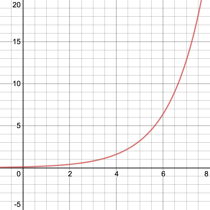
This graph is not a line, but rather a curve that slopes upward as it goes. Graphically, this means that exponential growth functions increase at an increasing rate. Linear functions, on the other hand, increase at a constant rate. This is the fundamental difference between linear and exponential functions.
Exponential Functions in Context
Exponential functions are used to describe many different real-world situations. Any situation in which there is a constant percent rate of change can be described using an exponential function. If the function is increasing, the percent rate of change will be positive, and the situation will be modeled using exponential growth. If the function is decreasing, the percent rate of change will be negative, and the situation will modeled using exponential decay. We will see an example of each scenario.
You are hired at a new job (congratulations!). Your starting salary is \(\$38,000\), and you are promised a raise of \(2.5\%\) per year. Write a function \(S(t)\) that describes your salary \(t\) years after starting the job. How much will you make \(4\) years after starting the job? How about \(5\) years after starting the job? And what is the percent change between these values?
Solution
We see that this situation has an initial value and a consistent percent change. Therefore, it must be an exponential function. As in previous sections, we can be flexible about the variable names we use in our functions. This question is asking for a function \(S(t)\), so we will use \(S\) in place of \(f\) and \(t\) in place of \(x\) in our generic exponential format. This helps us keep track of the fact that our input variable is time \(t\), and our output is \(S(t)\), the salary after \(t\) years. So, our function will have the format:\[S(t) = a(1+r)^t\] where \(a\) is the initial value and \(r\) is the percent rate of change. Since you start with a salary of \(\$38,000\), we have \(a = 38000\). Since there is a growth of \(2.5\%\) per year, we have \(r = .025\). Thus, our exponential function is: \[S(t) = 38000 (1+.025)^t\]
We can add the numbers in parentheses to simplify slightly. And in fact, this will help us more easily calculate using this function. That is, we can write \[S(t) = 38000(1.025)^t\]
Now, to find your salary \(4\) years after you start working, simply plug \(t = 4\) into the equation: \[S(t) = 38000 (1.025)^4 = 41944.89\]
Make sure, when checking the answer above, that you perform the exponent operation before multiplying by the initial value. Therefore, your salary after \(4\) years will be \(\$41,944.89\). We are rounding to two decimal points because this is an amount of money.
We can use a similar process to find the salary after 5 years. We have: \[ S(5) = 38000(1.025)^ 5 = 42993.51\]
Therefore, your salary after \(5\) years will be \(\$42,993.51\).
To find the percent change between these quantities, we remember from Chapter 2 that the percent change formula is given by \[\text{ percent change } = \frac{Q_2 - Q_1}{Q_1} \times 100\]
We'll use \(Q_1 = 41,944.89\) and \(Q_2 = 42,993.51\). Plugging in, we get \[\text{ percent change } = \frac{Q_2 - Q_1}{Q_1} \times 100 = \frac{42993.51 - 41944.89}{41944.89} \times 100 \approx 2.49999\]
Note that this is almost exactly \(2.5\%\). The very small error is due to the fact that we rounded the salaries to two decimal places. This confirms that our constant percent change persists year after year in this function.
The previous example shows a very straightforward application of the exponential function formula. We are presented with a percent change and an initial value, and we can simply write down the function and then use it.
A variation on this theme occurs when an exponential function is decreasing rather than increasing.
A new car costs \(\$35,000\) and its value depreciates at a rate of \(12\%\) each year. Find the formula \(V(t)\) that describes the value of a new car \(t\) years after you buy it. Find \(V(t)\) and interpret your answer in the context of a problem using a complete sentence.
Solution
The key word to understanding this questions is "depreciates." Something depreciates if it loses value over time. Many large purchases, such as cars, boats, and industrial equipment, depreciate over time. In fact, one of the tasks that accountants face is determining how to calculate depreciation for objects over time so they can determine the entire value of a person's or company's possessions at a given time. In this situation we will use a relatively simplistic model of depreciation, in which value decreases by a fixed percentage each year.
Since this is a situation involving a decreasing quantity, we need to choose \(r\) to be negative here. The percent change will therefore be \(-12\%\), or \(-.12\). The initial value remains positive, so we have \(a = 35000\). If we call our function \(V(t)\) for the value of the car at time \(t\), we have: \[V(t) = 35000(1+ (-.12))^t\]
which we can simplify as \[V(t) = 35000(.88)^t\]
From this form, we can view this situation slightly differently. The \(.88\) in parentheses indicates that the car retains \(88\%\) of its value from year to year. This is equivalent to losing \(12\%\) of its value. (This is a very similar method to what we used to calculate markdowns in Chapter 2.) Some folks find it easier to think about depreciation in this way.
In any case, now that we have our formula, we can find \(V(10)\): \[ V(10) = 35000 (.88)^{10} = 9747.53 \]
This means that, after \(10\) years, the car will be worth \(\$9,747.53\).
These two examples just brush the surface of the utility of exponential functions. In the next two sections, we'll investigate how exponential functions are used in financial mathematics.
Exercises
In these exercises, make sure to round all dollar amounts to two decimal places.
- Find a real-life situation that is modeled using either exponential growth or decay. Explain the situation in 1-2 sentences. If you use a source, please be sure to include a URL or other citation.
- A population of bacteria in an experiment is modeled by the function \(P(t) = 200(1.13)^t\) where \(t\) is measured in hours and \(P(t)\) is the number of bacteria at time \(t\).
- How many bacteria are there in the population at the start of the study?
- By what percentage does the population increase each hour?
- Find \(P(5)\) and round to the nearest whole. Then interpret your answer in the context of the problem, using a complete sentence.
- You want to save money. You start with \(\$100\) in your piggy bank, and you vow to increase the amount of money in your piggy bank by \(10\%\) each week. Write a function that describes the amount of money in your piggy bank after t weeks. How much will you have after one year? (Assume there are \(52\) weeks in a year.)
- A restaurant buys an industrial-size freezer. The freezer cost \(\$10,000\) new, and is estimated to have a depreciation rate of \(3.1\%\) per year. In \(15\) years, at what price should the restaurant value the freezer?