
11.1: Modelling the Eye


- Last updated
- Jul 4, 2022
- Save as PDF

( \newcommand{\kernel}{\mathrm{null}\,}\)
Let me model the temperature in a simple model of the eye, where the eye is a sphere, and the eyelids are circular. In that case we can put the z-axis straight through the middle of the eye, and we can assume that the temperature does only depend on r,θ and not on ϕ. We assume that the part of the eye in contact with air is at a temperature of 20∘ C, and the part in contact with the body is at 36∘ C.
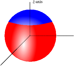
Figure 11.1.1: The temperature on the outside of a simple model of the eye
If we look for the steady state temperature it is described by Laplace’s equation,
∇2u(r,θ)=0.
Expressing the Laplacian ∇2 in spherical coordinates (see chapter 7) we find
1r2∂∂r (r2∂∂ru)+1r2sinθ∂∂θ (sinθ∂∂θu)=0.
Once again we solve the equation by separation of variables,
u(r,θ)=R(r)T(θ).
After this substitution we realize that
[r2R′]′R=−[sinθT′]′Tsinθ=λ.
The equation for R will be shown to be easy to solve (later). The one for T is of much more interest. Since for 3D problems the angular dependence is more complicated, whereas in 2D the angular functions were just sines and cosines.
The equation for T is
[sinθT′]′+λTsinθ=0.
This equation is called Legendre’s equation, or actually it carries that name after changing variables to x=cosθ. Since θ runs from 0 to π, we find sinθ>0, and we have
sinθ=√1−x2.
After this substitution we are making the change of variables we find the equation (y(x)=T(θ)=T(arccosx), and we now differentiate w.r.t. x, d/dθ=−√1−x2d/dx)
ddx[(1−x2)dydx]+λy=0.
This equation is easily seen to be self-adjoint. It is not very hard to show that x=0 is a regular (not singular) point – but the equation is singular at x=±1. Near x=0 we can solve it by straightforward substitution of a Taylor series,
y(x)=∑j=0ajxj.
We find the equation
∞∑j=0j(j−1)ajxj−2−∞∑j=0j(j−1)ajxj−2∞∑j=0jajxj+λ∞∑j=0ajxj=0
After introducing the new variable i=j−2, we have
∞∑j=0(i+1)(i+1)ai+2xi−∞∑j=0[j(j+1)−λ]ajxj=0.
Collecting the terms of the order xk, we find the recurrence relation ak+2=k(k+1)−λ(k+1)(k+2)ak.
If λ=n(n+1) this series terminates – actually those are the only acceptable solutions, any one where λ takes a different value actually diverges at x=+1 or x=−1, not acceptable for a physical quantity – it can’t just diverge at the north or south pole (x=cosθ=±1 are the north and south pole of a sphere).
We thus have, for n even,
yn=a0+a2x2+…+anxn.
For odd n we find odd polynomials,
yn=a1x+a3x3+…+anxn.
One conventionally defines an=(2n)!n!22n.
With this definition we obtain
P0=1, P1=x,P2=32x2−12,P3=12(5x3−3x),P4=18(35x4−30x2+3),P5=18(63x5−70x3+15x).
A graph of these polynomials can be found in figure 11.1.2.
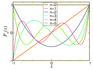
Figure 11.1.2: The first few Legendre polynomials Pn(x).