5.5: More Complex Initial/Boundary Conditions

It is not always possible on separation of variables to separate initial or boundary conditions in a condition on one of the two functions. We can either map the problem into simpler ones by using superposition of boundary conditions, a way discussed below, or we can carry around additional integration constants.

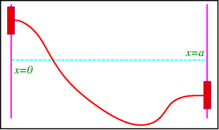
Let me give an example of these procedures. Consider a vibrating string attached to two air bearings, gliding along rods 4m apart. You are asked to find the displacement for all times, if the initial displacement, i.e. at \(t=0\)s is one meter and the initial velocity is \(x/t_0~\rm m/s\).

The differential equation and its boundary conditions are easily written down,

\[\begin{aligned} \dfrac{\partial^2}{\partial x^2} u &= \frac{1}{c^2} \dfrac{\partial^2}{\partial t^2} u ,\nonumber\\ \dfrac{\partial}{\partial x} u(0,t) &= \dfrac{\partial}{\partial x} u(4,t) = 0, \;t>0, \nonumber\\ u(x,0) & = 1, \nonumber\\ \dfrac{\partial}{\partial t} u(x,0) & = x /t_0.\end{aligned} \nonumber \]

Exercise \(\PageIndex{1}\)

What happens if I add two solutions \(v\) and \(w\) of the differential equation that satisfy the same BC’s as above but different IC’s,

\[\begin{aligned} v(x,0) =0 &,& \dfrac{\partial}{\partial t} v(x,0) = x /t_0, \nonumber\\ w(x,0) =1 &,& \dfrac{\partial}{\partial t} w(x,0) = 0?\end{aligned} \nonumber \]

Answer

\(u\)=\(v+w\), we can add the BC’s.

If we separate variables, \(u(x,t) = X(x)T(t)\), we find that we obtain easy boundary conditions for \(X(x)\), \[X'(0)=X'(4) = 0, \nonumber \] but we have no such luck for \((t)\). As before we solve the eigenvalue equation for \(X\), and find solutions for \(\lambda_n=\frac{n^2\pi^2}{16}\), \(n=0,1,...\), and \(X_n=\cos(\frac{n\pi}{4}x)\). Since we have no boundary conditions for \(T(t)\), we have to take the full solution,

\[\begin{aligned} T_0(t) &= A_0 + B_0 t, \nonumber\\ T_n(t) &= A_n \cos \frac{n\pi}{4} ct + B_n \sin \frac{n\pi}{4} ct,\end{aligned} \nonumber \] and thus \[u(x,t) = \dfrac{1}{2}(A_0 + B_0 t ) + \sum_{n=1}^\infty \left(A_n \cos \frac{n\pi}{4} ct + B_n \sin \frac{n\pi}{4} ct\right) \cos \frac{n\pi}{4}x. \nonumber \]

Now impose the initial conditions

• \[u(x,0) = 1 = \dfrac{1}{2} A_0 + \sum_{n=1}^\infty A_n \cos \frac{n\pi}{4}x, \nonumber \] which implies \(A_0=2\), \(A_n=0, n>0\).
• \[\dfrac{\partial}{\partial t} u(x,0) = x/t_0 = \dfrac{1}{2} B_0 + \sum_{n=1}^\infty \frac{n\pi c}{4} B_n \cos \frac{n\pi}{4}x. \nonumber \] This is the Fourier sine-series of \(x\), which we have encountered before, and leads to the coefficients \(B_0=4\) and \(B_n= -\frac{64}{n^3\pi^3c}\) if \(n\) is odd and zero otherwise.

So finally \[u(x,t) = (1+2t) -\frac{64}{\pi^3} \sum_{n~\rm odd} \frac{1}{n^3} \sin \frac{n\pi ct}{4 } \cos \frac{n\pi x}{4}. \nonumber \]