5.4: Laplace’s Equation

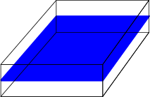
Figure $\PageIndex{1}$: A conducting sheet insulated from above and below.

In a square, heat-conducting sheet, insulated from above and below

$$\frac{1}{k}\dfrac{\partial}{\partial t} u = \dfrac{\partial^2}{\partial x^2} u + \dfrac{\partial^2}{\partial y^2} u. \nonumber$$

If we are looking for a steady state solution, i.e., we take $u(x,y,t)=u(x,y)$ the time derivative does not contribute, and we get Laplace’s equation

$$\dfrac{\partial^2}{\partial x^2} u + \dfrac{\partial^2}{\partial y^2} u=0, \nonumber$$

an example of an elliptic equation. Let us once again look at a square plate of size $a\times b$, and impose the boundary conditions

$$\begin{align} u(x,0) & = 0, \nonumber\\ u(a,y) & = 0, \nonumber\\ u(x,b) & = x, \nonumber\\ u(0,y) & = 0.\end{align} \nonumber$$

(This choice is made so as to be able to evaluate Fourier series easily. It is not very realistic!) We once again separate variables,

$$u(x,y) = X(x) Y(y), \nonumber$$

and define

$$\frac{X''}{X} = -\frac{Y''}{Y} = -\lambda. \nonumber$$

or explicitly

$$X'' = -\lambda X,\;\;Y''=\lambda Y. \nonumber$$

With boundary conditions $X(0)=X(a)=0$, $Y(0)=0$. The 3rd boundary conditions remains to be implemented.

Once again distinguish three cases:

$\lambda>0$

$X(x) = \sin \alpha_n(x)$, $\alpha_n=\frac{n\pi}{a}$, $\lambda_n=\alpha_n^2$. We find

$$\begin{align} Y(y) &= C_n\sinh \alpha_n y + D_n \cosh \alpha _n y \nonumber\\[4pt] &= C'_n\exp (\alpha_n y) + D'_n \exp(- \alpha _n y).\end{align} \nonumber$$

Since $Y(0)=0$ we find $D_n=0$ ($\sinh(0)=0,\cosh(0)=1$).

$\lambda \leq 0$

No solutions

So we have

$$u(x,y) = \sum_{n=1}^\infty b_n \sin\alpha_n x \sinh \alpha_n y \nonumber$$

The one remaining boundary condition gives

$$u(x,b) = x = \sum_{n=1}^\infty b_n \sin\alpha_n x \sinh \alpha_n b. \nonumber$$

This leads to the Fourier series of $x$,

$$\begin{align} b_n \sinh \alpha_n b &= \frac{2}{a} \int_0^a x \sin \frac{n\pi x}{a}dx \nonumber\\ &= \frac{2 a }{n\pi}(-1)^{n+1}.\end{align} \nonumber$$

So, in short, we have

$$V(x,y) = \frac{2a}{\pi} \sum_{n=1}^\infty (-1)^{n+1} \frac{\sin \frac{n\pi x}{a}\sinh \frac{n\pi y}{a}}{n \sinh \frac{n\pi b}{a}}. \nonumber$$

Exercise $\PageIndex{1}$

The dependence on $x$ enters through a trigonometric function, and that on $y$ through a hyperbolic function. Yet the differential equation is symmetric under interchange of $x$ and $y$. What happens?

Answer

The symmetry is broken by the boundary conditions.