9.7: The Laplace Equation

The diffusion equation in two spatial dimensions is \[u_t=D(u_{xx}+u_{yy}).\nonumber\]

The steady-state solution, approached asymptotically in time, has \(u_t = 0\) so that the steady-state solution \(u = u(x, y)\) satisfies the two-dimensional Laplace equation \[\label{eq:1}u_{xx}+u_{yy}=0.\]

We will consider the mathematical problem of solving the two dimensional Laplace equation inside a rectangular or a circular boundary. The value of \(u(x, y)\) will be specified on the boundaries, defining this problem to be of Dirichlet type.

Dirichlet Problem for a Rectangle

Figure \(\PageIndex{1}\): Dirichlet problem for the Laplace equation in a rectangle.

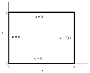
We consider the Laplace equation \(\eqref{eq:1}\) for the interior of a rectangle \(0 < x < a\), \(0 < y < b\), (see Fig. \(\PageIndex{1}\)), with boundary conditions \[\begin{array}{lllll}u(x,0)=0, && u(x,b)=0, && 0<x<a; \\ u(0,y)=0, && u(a,y)=f(y),&& 0\leq y\leq b.\end{array}\nonumber\]

More general boundary conditions can be solved by linear superposition of solutions.

We take our usual ansatz \[u(x,y)=X(x)Y(y),\nonumber\] and find after substitution into \(\eqref{eq:1}\), \[\frac{X''}{X}=-\frac{Y''}{Y}=\lambda,\nonumber\] with \(\lambda\) the separation constant. We thus obtain the two ordinary differential equations \[X''-\lambda X=0,\quad Y''+\lambda Y=0.\nonumber\]

The homogeneous boundary conditions are \(X(0) = 0,\: Y(0) = 0\) and \(Y(b) = 0\). We have already solved the equation for \(Y(y)\) in §9.5, and the solution yields the eigenvalues \[\lambda_n=\left(\frac{n\pi}{b}\right)^2,\quad n=1,2,3,\ldots ,\nonumber\] with corresponding eigenfunctions \[Y_n(y)=\sin\frac{n\pi y}{b}.\nonumber\]

The remaining \(X\) equation and homogeneous boundary condition is therefore \[X''-\frac{n^2\pi^2}{b^2}X=0,\quad X(0)=0,\nonumber\] and the solution is the hyperbolic sine function \[X_n(x)=\sinh\frac{n\pi x}{b},\nonumber\] times a constant. Writing \(u_n = X_nY_n\), multiplying by a constant and summing over \(n\), yields the general solution \[u(x,y)=\sum\limits_{n=0}^\infty c_n\sinh\frac{n\pi x}{b}\sinh\frac{n\pi y}{b}.\nonumber\]

The remaining inhomogeneous boundary condition \(u(a, y) = f(y)\) results in \[f(y)=\sum\limits_{n=0}^\infty c_n\sinh\frac{n\pi a}{b}\sin\frac{n\pi y}{b},\nonumber\] which we recognize as a Fourier sine series for an odd function with period \(2b\), and coefficient \(c_n \sinh (n\pi a/b)\). The solution for the coefficient is given by \[c_n=\frac{2}{b\sinh\frac{n\pi a}{b}}\int_0^b f(y)\sin\frac{n\pi y}{b}dy.\nonumber\]

Dirichlet Problem for a Circle

The Laplace equation is commonly written symbolically as \[\label{eq:2}\nabla ^2u=0,\] where \(\nabla^2\) is called the Laplacian, sometimes denoted as \(\Delta\). The Laplacian can be written in various coordinate systems, and the choice of coordinate systems usually depends on the geometry of the boundaries. Indeed, the Laplace equation is known to be separable in \(13\) different coordinate systems! We have solved the Laplace equation in two dimensions, with boundary conditions specified on a rectangle, using \[\nabla ^2=\frac{\partial ^2}{\partial x^2}+\frac{\partial ^2}{\partial y^2}.\nonumber\]

Here we consider boundary conditions specified on a circle, and write the Laplacian in polar coordinates by changing variables from cartesian coordinates. Polar coordinates is defined by the transformation \((r,\theta )\to (x, y)\):

\[\label{eq:3}x=r\cos\theta,\quad y=r\sin\theta ;\] and the chain rule gives for the partial derivatives \[\label{eq:4}\frac{\partial u}{\partial r}=\frac{\partial u}{\partial x}\frac{\partial x}{\partial r}+\frac{\partial u}{\partial y}\frac{\partial y}{\partial r},\quad \frac{\partial u}{\partial\theta}=\frac{\partial u}{\partial x}\frac{\partial x}{\partial\theta}+\frac{\partial u}{\partial y}\frac{\partial y}{\partial\theta}.\]

After taking the partial derivatives of \(x\) and \(y\) using \(\eqref{eq:3}\), we can write the transformation \(\eqref{eq:4}\) in matrix form as \[\label{eq:5}\left(\begin{array}{c}\partial u/\partial r \\ \partial u/\partial\theta\end{array}\right)=\left(\begin{array}{rr}\cos\theta &\sin\theta \\ -r\sin\theta & r\cos\theta\end{array}\right)\left(\begin{array}{c}\partial u/\partial x \\ \partial u/\partial y\end{array}\right).\]

Inversion of \(\eqref{eq:5}\) can be determined from the following result, commonly proved in a linear algebra class. If \[A=\left(\begin{array}{cc}a&b \\ c&d\end{array}\right),\quad\det A\neq 0,\nonumber\] then \[A^{-1}=\frac{1}{\det A}\left(\begin{array}{cc}d&-b \\ -c&a\end{array}\right).\nonumber\]

Therefore, since the determinant of the \(2\times 2\) matrix in \(\eqref{eq:5}\) is \(r\), we have \[\label{eq:6}\left(\begin{array}{c}\partial u/\partial x \\ \partial u/\partial y\end{array}\right)=\left(\begin{array}{rr}\cos\theta &-\sin\theta /r \\ \sin\theta &\cos\theta /r\end{array}\right)\left(\begin{array}{c}\partial u/\partial r \\ \partial u/\partial\theta\end{array}\right).\]

Rewriting \(\eqref{eq:6}\) in operator form, we have \[\label{eq:7}\frac{\partial}{\partial x}=\cos\theta\frac{\partial}{\partial r}-\frac{\sin\theta}{r}\frac{\partial}{\partial\theta},\quad\frac{\partial}{\partial y}=\sin\theta\frac{\partial}{\partial r}+\frac{\cos\theta}{r}\frac{\partial}{\partial\theta}.\]

To find the Laplacian in polar coordinates with minimum algebra, we combine \(\eqref{eq:7}\) using complex variables as \[\label{eq:8}\frac{\partial}{\partial x}+i\frac{\partial}{\partial y}=e^{i\theta}\left(\frac{\partial}{\partial r}+\frac{i}{r}\frac{\partial}{\partial\theta}\right),\] so that the Laplacian may be found by multiplying both sides of \(\eqref{eq:8}\) by its complex conjugate, taking care with the computation of the derivatives on the righthand-side:

\[\begin{aligned}\frac{\partial ^2}{\partial x^2}+\frac{\partial ^2}{\partial y^2}&=e^{i\theta}\left(\frac{\partial}{\partial r}+\frac{i}{r}\frac{\partial}{\partial\theta}\right)e^{-i\theta}\left(\frac{\partial}{\partial r}-\frac{1}{r}\frac{\partial}{\partial\theta}\right) \\ &=\frac{\partial ^2}{\partial r^2}+\frac{1}{r}\frac{\partial }{\partial r}+\frac{1}{r^2}\frac{\partial ^2}{\partial\theta ^2}.\end{aligned}\]

We have therefore determined that the Laplacian in polar coordinates is given by \[\label{eq:9}\nabla^2=\frac{\partial ^2}{\partial r^2}+\frac{1}{r}\frac{\partial }{\partial r}+\frac{1}{r^2}\frac{\partial ^2}{\partial\theta^2},\] which is sometimes written as \[\nabla^2 =\frac{1}{r}\frac{\partial}{\partial r}\left(r\frac{\partial}{\partial r}\right)+\frac{1}{r^2}\frac{\partial ^2}{\partial\theta ^2}.\nonumber\]

We now consider the solution of the Laplace equation in a circle with radius \(r < a\) subject to the boundary condition \[\label{eq:10}u(a,\theta )=f(\theta),\quad 0\leq\theta\leq 2\pi.\]

An additional boundary condition due to the use of polar coordinates is that \(u(r, \theta )\) is periodic in \(\theta\) with period \(2\pi\). Furthermore, we will also assume that \(u(r, \theta )\) is finite within the circle.

The method of separation of variables takes as our ansatz \[u(r,\theta )=R(r)\Theta (\theta ),\nonumber\] and substitution into the Laplace equation \(\eqref{eq:2}\) using \(\eqref{eq:9}\) yields \[R''\Theta +\frac{1}{r}R'\Theta +\frac{1}{r^2}R\Theta ''=0,\nonumber\] or \[r^2\frac{R''}{R}+r\frac{R'}{R}=-\frac{\Theta ''}{\Theta }=\lambda,\nonumber\] where \(\lambda\) is the separation constant. We thus obtain the two ordinary differential equations \[r^2R''+rR'-\lambda R=0,\quad \Theta ''+\lambda\Theta =0.\nonumber\]

The \(\Theta\) equation is solved assuming periodic boundary conditions with period \(2\pi\). If \(\lambda < 0\), then no periodic solution exists. If \(\lambda = 0\), then \(\Theta\) can be constant. If \(\lambda = \mu^2 > 0\), then \[\Theta (\theta )=A\cos\mu\theta +B\sin\mu\theta ,\nonumber\] and the requirement that \(\Theta\) is periodic with period \(2\pi\) forces \(\mu\) to be an integer. Therefore, \[\lambda_n=n^2,\quad n=0,1,2,\ldots ,\nonumber\] with corresponding eigenfunctions \[\Theta_n(\theta )=A_n\cos n\theta +B_n\sin n\theta.\nonumber\]

The \(R\) equation for each eigenvalue \(\lambda_n\) then becomes \[\label{eq:11}r^2R''+rR'-n^2R=0,\] which is an Euler equation. With the ansatz \(R = r^s\), \(\eqref{eq:11}\) reduces to the algebraic equation \(s(s − 1) + s − n^2 = 0\), or \(s^2 = n^2\). Therefore, \(s = ±n\), and there are two real solutions when \(n > 0\) and degenerate solutions when \(n = 0\). When \(n > 0\), the solution for \(R(r)\) is \[R_n(r)=Ar^n+Br^{-n}.\nonumber\]

The requirement that \(u(r,\theta )\) is finite in the circle forces \(B = 0\) since \(r^{−n}\) becomes unbounded as \(r\to 0\). When \(n = 0\), the solution for \(R(r)\) is \[R_n(r)=A+B\ln r,\nonumber\] and again finite \(u\) in the circle forces \(B = 0\). Therefore, the solution for \(n = 0,\: 1,\: 2,\ldots\) is \(R_n = r^n\). Thus the general solution for \(u(r,\theta )\) may be written as \[\label{eq:12} u(r,\theta )=\frac{A_0}{2}+\sum\limits_{n=1}^\infty r^n (A_n\cos n\theta +B_n\sin n\theta ),\] where we have separated out the \(n = 0\) solution to write our solution in a form similar to the standard Fourier series given by (9.3.1). The remaining boundary condition \(\eqref{eq:10}\) specifies the values of u on the circle of radius a, and imposition of this boundary condition results in \[\label{eq:13} f(\theta )=\frac{A_0}{2}+\sum\limits_{n=1}^\infty a^n (A_n\cos n\theta +B_n\sin n\theta ).\]

Equation \(\eqref{eq:13}\) is a Fourier series for the periodic function \(f(\theta )\) with period \(2\pi\), i.e., \(L = \pi\) in (9.3.1). The Fourier coefficients \(a^nA_n\) and \(a^nB_n\) are therefore given by (9.3.5) and (9.3.6) to be \[\begin{align} a^nA_n&=\frac{1}{\pi}\int_0^{2\pi} f(\phi )\cos n\phi d\phi, \quad n=0,1,2,\ldots ; \nonumber \\ a^nB_n&=\frac{1}{\pi}\int_0^{2\pi}f(\phi )\sin n\phi d\phi ,\quad n=1,2,3,\ldots ,\label{eq:14}\end{align}\] where we have used \(\phi\) for the dummy variable of integration.

A remarkable fact is that the infinite series solution for \(u(r, \theta )\) can be summed explicitly. Substituting \(\eqref{eq:14}\) into \(\eqref{eq:12}\), we obtain \[\begin{aligned}u(r,\theta )&=\frac{1}{2\pi}\int_0^{2\pi}d\phi f(\phi )\left[ 1+2\sum\limits_{n=1}^\infty \left(\frac{r}{a}\right)^n (\cos n\theta\cos n\phi +\sin n\theta\sin n\phi )\right] \\ &=\frac{1}{2\pi}\int_0^{2\pi} d\phi f(\phi)\left[1+2\sum_{n=1}^\infty \left(\frac{r}{a}\right)^n\cos n(\theta -\phi)\right].\end{aligned}\]

We can sum the infinite series by writing \(2 cos n(\theta − \phi ) = e^{in(\theta−\phi)} + e^{−in(\theta −\phi)}\), and using the sum of the geometric series \(\sum_{n=1}^\infty z^n = z/(1 − z)\) to obtain \[\begin{aligned} 1+2\sum\limits_{n=1}^\infty \left(\frac{r}{a}\right)^n\cos n(\theta -\phi)&=1+\sum\limits_{n=1}^\infty \left(\frac{re^{i(\theta -\phi)}}{a}\right)^n +\sum\limits_{n=1}^\infty \left(\frac{re^{-i(\theta -\phi )}}{a}\right)^n \\ &=1+\left(\frac{re^{i(\theta -\phi)}}{a-re^{i(\theta -\phi )}}+c.c.\right) \\ &=\frac{a^2-r^2}{a^2-2ar\cos (\theta -\phi )+r^2}.\end{aligned}\]

Therefore, \[u(r,\theta )=\frac{a^2-r^2}{2\pi}\int_0^{2\pi}\frac{f(\phi )}{a^2-2ar\cos (\theta -\phi )+r^2}d\phi,\nonumber\] an integral result for \(u(r, \theta )\) known as Poisson’s formula. As a trivial example, consider the solution for \(u(r, \theta )\) if \(f(\theta ) = F\), a constant. Clearly, \(u(r, \theta ) = F\) satisfies both the Laplace equation and the boundary conditions so must be the solution. You can verify that \(u(r, \theta ) = F\) is indeed the solution by showing that \[\int_0^{2\pi}\frac{d\phi}{a^2-2ar\cos (\theta -\phi )+r^2}=\frac{2\pi }{a^2-r^2}.\nonumber\]