9.8: The Schrödinger Equation

The Schrödinger equation is the equation of motion for nonrelativistic quantum mechanics. This equation is a linear partial differential equation and in simple situations can be solved using the technique of separation of variables. Luckily, one of the cases that can be solved analytically is the hydrogen atom. It can be argued that the greatest success of classical mechanics was the solution of the Earth-Sun system. Similarly, it can be argued that the greatest success of quantum mechanics was the solution of the electron-proton system. The mathematical solutions of these classical and quantum two-body problems rank among the highest achievements of mankind.

Heuristic Derivation of the Schrödinger Equation

Nature consists of waves and particles. Early in the twentieth century, light was discovered to act as both a wave and a particle, and quantum mechanics assumes that matter can also act in both ways.

In general, waves are described by their wavelength \(\lambda\) and frequency \(ν\), or equivalently their wavenumber \(k = 2\pi /\lambda\) and their angular frequency \(\omega = 2\pi ν\). The Planck-Einstein relations for light postulated that the energy \(E\) and momentum \(p\) of a light particle, called a photon, is proportional to the angular frequency \(\omega\) and wavenumber \(k\) of the light wave. The proportionality constant is called “h bar”, denoted as \(\overline{h}\), and is related to the original Planck’s constant h by \(\overline{h} = h/2\pi\). The Planck-Einstein relations are given by \[E=\overline{h}\omega ,\quad p=\overline{h}k.\nonumber\]

De Broglie in 1924 postulated that matter also follows these relations.

A heuristic derivation of the Schrödinger equation for a particle of mass \(m\) and momentum \(p\) constrained to move in one dimension begins with the classical equation \[\label{eq:1}\frac{p^2}{2m}+V(x,t)=E,\] where \(p^2/2m\) is the kinetic energy of the mass, \(V(x, t)\) is the potential energy, and \(E\) is the total energy.

In search of a wave equation, we consider how to write a free wave in one dimension. Using a real function, we could write \[\label{eq:2}\Psi =A\cos (kx-\omega t+\phi ),\] where \(A\) is the amplitude and \(\phi\) is the phase. Or using a complex function, we could write \[\label{eq:3}\Psi =Ce^{i(kx-\omega t)},\] where \(C\) is a complex number containing both amplitude and phase.

We now rewrite the classical energy equation \(\eqref{eq:1}\) using the Planck-Einstein relations. After multiplying by a wavefunction, we have \[\frac{\overline{h}^2}{2m}k^2\Psi (x,t)+V(x,t)\Psi (x,t)=\overline{h}\omega\Psi (x,t).\nonumber\]

We would like to replace \(k\) and \(\omega\), which refer to the wave characteristics of the particle, by differential operators acting on the wavefunction \(\Psi (x, t)\). If we consider \(V(x, t) = 0\) and the free particle wavefunctions given by \(\eqref{eq:2}\) and \(\eqref{eq:3}\), it is easy to see that to replace both \(k^2\) and \(\omega\) by derivatives we need to use the complex form of the wavefunction and explicitly introduce the imaginary unit \(i\), that is \[k^2\to -\frac{\partial ^2}{\partial x^2},\quad\omega\to i\frac{\partial}{\partial t}.\nonumber\]

Doing this, we obtain the intrinsically complex equation \[-\frac{\overline{h}^2}{2m}\frac{\partial ^2\Psi}{\partial x^2}+V(x,t)\Psi =i\overline{h}\frac{\partial\Psi}{\partial t},\nonumber\] which is the one-dimensional Schrödinger equation for a particle of mass \(m\) in a potential \(V = V(x, t)\). This equation is easily generalized to three dimensions and takes the form \[\label{eq:4} -\frac{\overline{h}^2}{2m}\nabla ^2\Psi (\mathbf{x},\mathbf{t})+V(\mathbf{x},t)\Psi (\mathbf{x},t)=i\overline{h}\frac{\partial\Psi (\mathbf{x},t)}{\partial t},\] where in Cartesian coordinates the Laplacian \(\nabla^2\) is written as \[\nabla^2=\frac{\partial ^2}{\partial x^2}+\frac{\partial^2}{\partial y^2}+\frac{\partial ^2}{\partial z^2}.\nonumber\]

The Born interpretation of the wavefunction states that \(|\Psi (\mathbf{x}, t)|^2\) is the probability density function of the particle’s location. That is, the spatial integral of \(|\Psi (\mathbf{x}, t)|^2\) over a volume \(V\) gives the probability of finding the particle in \(V\) at time \(t\). Since the particle must be somewhere, the wavefunction for a bound particle is usually normalized so that \[\int_{-\infty}^\infty \int_{-\infty}^\infty \int_{-\infty}^\infty |\Psi (x,y,z;t)|^2dx\:dy\:dz =1.\nonumber\]

The simple requirements that the wavefunction be normalizable as well as single valued admits an analytical solution of the Schrödinger equation for the hydrogen atom.

The Time-Independent Schrödinger Equation

The space and time variables of the time-dependent Schrödinger equation \(\eqref{eq:4}\) can be separated provided the potential function \(V(\mathbf{x}, t) = V(\mathbf{x})\) is independent of time. We try \(\Psi (\mathbf{x}, t) = \psi (x)f(t)\) and obtain \[-\frac{\overline{h}^2}{2m}f\nabla ^2\psi +V(\mathbf{x})\psi f=i\overline{h}\psi f'.\nonumber\]

Dividing by \(\psi f\), the equation separates as \[-\frac{\overline{h}^2}{2m}\frac{\nabla ^2\psi}{\psi}+V(\mathbf{x})=i\overline{h}\frac{f'}{f}.\nonumber\]

The left-hand side is independent of \(t\), the right-hand side is independent of \(\mathbf{x}\), so both the left- and right-hand sides must be independent of \(\mathbf{x}\) and \(t\) and equal to a constant. We call this separation constant \(E\), thereby reintroducing the total energy into the equation. We now have the two differential equations \[f'=-\frac{iE}{\overline{h}}f,\quad -\frac{\overline{h}^2}{2m}\nabla^2\psi +V(\mathbf{x})\psi =E\psi.\nonumber\]

The second equation is called the time-independent Schrödinger equation. The first equation can be easily integrated to obtain \[f(t)=e^{-iEt/\overline{h}},\nonumber\] which can be multiplied by a arbitrary constant.

Particle in a One-Dimensional Box

We assume that a particle of mass \(m\) is able to move freely in only one dimension and is confined to the region defined by \(0 < x < L\). This is perhaps the simplest quantum mechanical problem with quantized energy levels. We take as the potential energy function \[V(x)=\left\{\begin{array}{ll}0,& 0<x<L, \\ \infty ,&\text{otherwise},\end{array}\right.\nonumber\] where we may assume that the particle is forbidden from the region with infinite potential energy. We will simply take as the boundary conditions on the wavefunction \[\label{eq:5}\psi (0)=\psi (L)=0.\]

For this potential, the time-independent Schrödinger equation for \(0 < x < L\) reduces to \[-\frac{\overline{h}^2}{2m}\frac{d^2\psi}{dx^2}=E\psi ,\nonumber\] which we write in a familiar form as \[\label{eq:6}\frac{d^2\psi}{dx^2}+\left(\frac{2mE}{\overline{h}^2}\right)\psi =0.\]

Equation \(\eqref{eq:6}\) together with the boundary conditions \(\eqref{eq:5}\) form an ode eigenvalue problem, which is in fact identical to the problem we solved for the diffusion equation in subsection 9.5.

The general solution to this second-order differential equation is given by \[\psi (x)=A\cos\frac{\sqrt{2mE}x}{\overline{h}}+B\sin\frac{\sqrt{2mE}x}{\overline{h}}.\nonumber\]

The first boundary condition \(\psi (0) = 0\) yields \(A = 0\). The second boundary condition \(\psi (L) = 0\) yields \[\frac{\sqrt{2mE}L}{\overline{h}}=n\pi ,\quad n=1,2,3,\ldots\nonumber\]

The energy levels of the particle are therefore quantized, and the allowed values are given by \[E_n=\frac{n^2\pi^2\overline{h}^2}{2mL^2}.\nonumber\]

The corresponding wavefunction is given by \(\psi_n = B \sin (n\pi x/L)\). We can normalize each wavefunction so that \[\int_0^L |\psi_n(x)|^2 dx=1,\nonumber\] obtaining \(B=\sqrt{2/L}\). We have therefore obtained \[\psi_n(x)=\left\{\begin{array}{ll}\sqrt{\frac{2}{L}}\sin\frac{n\pi x}{L},&0<x<L; \\ 0,&\text{otherwise.}\end{array}\right.\nonumber\]

The Simple Harmonic Oscillator

Hooke’s law for a mass on a spring is given by \[F=-Kx,\nonumber\] where \(K\) is the spring constant. The potential energy \(V(x)\) in classical mechanics satisfies \[F=-\partial V/\partial x,\nonumber\] so that the potential energy of the spring is given by \[V(x)=\frac{1}{2}Kx^2.\nonumber\]

Recall that the differential equation for a classical mass on a spring is given from Newton’s law by \[m\overset{..}{x}=-Kx,\nonumber\] which can be rewritten as \[\overset{..}{x}+\omega^2x=0,\nonumber\] where \(\omega^2 = K/m\). Following standard notation, we will therefore write the potential energy as \[V(x)=\frac{1}{2}m\omega^2x^2.\nonumber\]

The time-independent Schrödinger equation for the one-dimensional simple harmonic oscillator then becomes \[\label{eq:7}-\frac{\overline{h}^2}{2m}\frac{d^2\psi}{dx^2}+\frac{1}{2}m\omega^2x^2\psi =E\psi .\]

The relevant boundary conditions are \(\psi\to 0\) as \(x\to ±\infty\) so that the wavefunction is normalizable.

The Schrödinger equation given by \(\eqref{eq:7}\) can be made neater by nondimensionalization. We rewrite \(\eqref{eq:7}\) as \[\label{eq:8}\frac{d^2\psi}{dx^2}+\left(\frac{2mE}{\overline{h}^2}-\frac{m^2\omega^2x^2}{\overline{h}^2}\right)\psi =0,\] and observe that the dimension \([\overline{h}^/m^2\omega^2 ] = l^4\), where \(l\) is a unit of length. We therefore let \[x=\sqrt{\frac{\overline{h}}{m\omega}}y,\quad\psi (x)=u(y),\nonumber\] and \(\eqref{eq:8}\) becomes \[\label{eq:9}\frac{d^2 u}{dy^2}+(\mathcal{E}-y^2)u=0,\] with the dimensionless energy given by \[\label{eq:10}\mathcal{E}=2E/\overline{h}\omega ,\] and boundary conditions \[\label{eq:11}\underset{y\to\pm\infty}{\lim}u(y)=0.\]

The dimensionless Schrödinger equation given by \(\eqref{eq:9}\) together with the boundary conditions \(\eqref{eq:11}\) forms another ode eigenvalue problem. A nontrivial solution for \(u = u(y)\) exists only for discrete values of \(\mathcal{E}\), resulting in the quantization of the energy levels. Since the second-order ode given by \(\eqref{eq:9}\) has a nonconstant coefficient, we can use the techniques of Chapter 6 to find a convergent series solution for \(u = u(y)\) that depends on \(\mathcal{E}\). However, we will then be faced with the difficult problem of determining the values of \(\mathcal{E}\) for which \(u(y)\) satisfies the boundary conditions \(\eqref{eq:11}\).

A path to an analytical solution can be discovered if we first consider the behavior of \(u\) for large values of \(y\). With \(y^2 >>\mathcal{E}\), \(\eqref{eq:9}\) reduces to \[\label{eq:12}\frac{d^2u}{dy^2}-y^2u=0.\]

To determine the behavior of \(u\) for large \(y\), we try the ansatz \[u(y)=e^{ay^2}.\nonumber\]

We have \[u'(y)=2aye^{ay^2},\nonumber\] \[u''(y)=e^{ay^2}\left(2a+4a^2y^2\right)\approx 4a^2y^2e^{ay^2},\nonumber\] and substitution into \(\eqref{eq:12}\) results in \[(4a^2-1)y^2=0,\nonumber\] yielding \(a = ±1/2\). Therefore at large \(y\), \(u(y)\) either grows like \(e^{y^2/2}\) or decays like \(e^{−y^2/2}\). Here, we have neglected a possible polynomial factor in front of the exponential functions. Clearly, the boundary conditions forbid the growing behavior and only allow the decaying behavior.

We proceed further by letting \[u(y)=H(y)e^{-y^2/2},\nonumber\] and determining the differential equation for \(H(y)\). After some simple calculation, we have \[u'(y)=(H'-yH)e^{-y^2/2},\quad u''(y)=\left(H''-2yH'+(y^2-1)H\right)e^{-y^2/2}.\nonumber\]

Substitution of the second derivative and the function into \(\eqref{eq:9}\) results in the differential equation \[\label{eq:13}H''-2yH'+(\mathcal{E}-1)H=0.\]

We now solve \(\eqref{eq:13}\) by a power-series ansatz. We try \[H(y)=\sum\limits_{k=0}^\infty a_ky^k.\nonumber\]

Substitution into \(\eqref{eq:13}\) and shifting indices as detailed in Chapter 6 results in \[\sum\limits_{k=0}^\infty ((k+2)(k+1)a_{k+2}+(\mathcal{E}-1-2k)a_k)y^k=0.\nonumber\]

We have thus obtained the recursion relation \[\label{eq:14}a_{k+2}=\frac{(1+2k)-\mathcal{E}}{(k+2)(k+1)}a_k,\quad k=0,1,2,\ldots\]

Now recall that apart from a possible multiplicative polynomial factor, \(u(y) ∼ e^{y^2/2}\) or \(e^{−y^2/2}\). Therefore, \(H(y)\) either goes like a polynomial times \(e^{y^2}\) or a polynomial. The function \(H(y)\) will be a polynomial only if \(\mathcal{E}\) takes on specific values which truncate the infinite power series.

Before we jump to this conclusion, I want to show that if the power series does not truncate, then \(H(y)\) does indeed grow like \(e^{y^2}\) for large \(y\). We first write the Taylor series for \(e^{y^2}\):

\[\begin{aligned}e^{y^2}&=1+y^2+\frac{y^4}{2!}+\frac{y^6}{3!}+\cdots \\ &=\sum\limits_{k=0}^\infty b_ky^k,\end{aligned}\] where \[b_k=\left\{\begin{array}{ll}\frac{1}{(k/2)!},&\text{n even;} \\ 0,&\text{k odd.}\end{array}\right.\nonumber\]

For large values of \(y\), the later terms of the power series dominate the earlier terms and the behavior of the function is determined by the large \(k\) coefficients. Provided \(k\) is even, we have \[\begin{aligned}\frac{b_{k+2}}{b_k}&=\frac{(k/2)!}{((k+2)/2)!} \\ &=\frac{1}{(k/2)+1} \\ &\sim \frac{2}{k}.\end{aligned}\]

The ratio of the coefficients would have been the same even if we had multiplied \(e^{y^2}\) by a polynomial.

The behavior of the coefficients for large \(k\) of our solution to the Schrödinger equation is given by the recursion relation \(\eqref{eq:14}\), and is \[\begin{aligned}\frac{a_{k+2}}{a_k}&=\frac{(1+2k)-\mathcal{E}}{(k+2)(k+1)} \\ &\sim\frac{2k}{k^2} \\ &=\frac{2}{k},\end{aligned}\] the same behavior as the Taylor series for \(e^{y^2}\). For large \(y\), then, the infinite power series for \(H(y)\) will grow as \(e^{y^2}\) times a polynomial. Since this does not satisfy the boundary conditions for \(u(y)\) at infinity, we must force the power series to truncate, which it does if we set \(\mathcal{E}=\mathcal{E}_n\), where \[\mathcal{E}_n=1+2n,\quad n=0,1,2,\ldots ,\nonumber\] resulting in quantization of the energy. The dimensional result is \[E_n=\overline{h}\omega (n+\frac{1}{2}),\nonumber\] with the ground state energy level given by \(E_0 =\overline{h}\omega/2\). The wavefunctions associated with each \(E_n\) can be determined from the power series and are the so-called Hermite polynomials times the decaying exponential factor. The constant coefficient can be determined by requiring the wavefunctions to integrate to one.

For illustration, the first two energy eigenfunctions, corresponding to the ground state and the first excited state, are given by \[\psi_0(x)=\left(\frac{m\omega}{\pi\overline{h}}\right)^{1/4}e^{-m\omega x^2/2\overline{h}},\quad \psi_1(x)=\left(\frac{m\omega}{\pi\overline{h}}\right)^{1/4}\sqrt{\frac{2m\omega}{\overline{h}}}xe^{-m\omega x^2/2\overline{h}}.\nonumber\]

Particle in a Three-Dimensional Box

To warm up to the analytical solution of the hydrogen atom, we solve what may be the simplest three-dimensional problem: a particle of mass \(m\) able to move freely inside a cube. Here, with three spatial dimensions, the potential is given by \[V(x,y,z)=\left\{\begin{array}{ll}0,&0<x,\: y,\: z<L, \\ \infty ,&\text{otherwise.}\end{array}\right.\nonumber\]

We may simply impose the boundary conditions \[\psi (0,y,z)=\psi(L,y,z)=\psi(x,0,z)=\psi(x,L,z)=\psi(x,y,0)=\psi(x,y,L)=0.\nonumber\]

The Schrödinger equation for the particle inside the cube is given by \[-\frac{\overline{h}^2}{2m}\left(\frac{\partial^2\psi}{\partial x^2}+\frac{\partial^2\psi}{\partial y^2}+\frac{\partial^2\psi}{\partial z^2}\right)=E\psi .\nonumber\]

We separate this equation by writing \[\psi (x,y,z)=X(x)Y(y)Z(z),\nonumber\] and obtain \[-\frac{\overline{h}^2}{2m}(X''YZ +XY''Z +XYZ'')=EXYZ.\nonumber\]

Dividing by \(XYZ\) and isolating the \(x\)-dependence first, we obtain \[-\frac{\overline{h}^2}{2m}\frac{X''}{X}=\frac{\overline{h}^2}{2m}\left(\frac{Y''}{Y}+\frac{Z''}{Z}\right)+E.\nonumber\]

The left-hand side is independent of \(y\) and \(z\) and the right-hand side is independent of \(x\) so that both sides must be a constant, which we call \(E_x\). Next isolating the \(y\)-dependence, we obtain \[-\frac{\overline{h}^2}{2m}\left(\frac{Y''}{Y}\right)=\frac{\overline{h}^2}{2m}\left(\frac{Z''}{Z}\right)+E-E_x.\nonumber\]

The left-hand side is independent of \(x\) and \(z\) and the right-hand side is independent of \(x\) and \(y\) so that both sides must be a constant, which we call \(E_y\). Finally, we define \(E_z = E − E_x − E_y\). The resulting three differential equations are given by \[X''+\frac{2mE_x}{\overline{h}^2}X=0,\quad Y''+\frac{2mE_y}{\overline{h}^2}Y=0,\quad Z''+\frac{2mE_z}{\overline{h}^2}Z=0.\nonumber\]

These are just three independent one-dimensional box equations so that the energy eigenvalue is given by \[E_{n_xn_yn_z}=\frac{(n_x^2+N_y^2+n_z^2)\pi^2\overline{h}^2}{2mL^2}.\nonumber\] and the associated wavefunction is given by \[\psi_{n_xn_yn_z}=\left\{\begin{array}{ll}\left(\frac{2}{L}\right)^{3/2}\sin\frac{n\pi x}{L}\sin\frac{n\pi y}{L}\sin\frac{n\pi z}{L},&0<x,\: y,\: z<L; \\ 0,&\text{otherwise.}\end{array}\right.\nonumber\]

The Hydrogen Atom

Hydrogen-like atoms, made up of a single electron and a nucleus, are the atomic two-body problems. As is also true for the classical two-body problem, consisting of say a planet and the Sun, the atomic two-body problem can be reduced to a one-body problem by transforming to center-of-mass coordinates and defining a

Figure \(\PageIndex{1}\): The spherical coordinate system, with radical distance \(r\), polar angle \(\theta\) and azimuthal angle \(\phi \).

reduced mass \(\mu\). We will not go into these details here, but will just take as the relevant Schrödinger equation \[\label{eq:15}-\frac{\overline{h}^2}{2\mu}\nabla^2\psi +V(r)\psi =E\psi ,\] where the potential energy \(V = V(r)\) is a function only of the distance \(r\) of the reduced mass to the center-of-mass. The explicit form of the potential energy from the electrostatic force between an electron of charge \(−e\) and a nucleus of charge \(+Ze\) is given by \[\label{eq:16}V(r)=-\frac{Ze^2}{4\pi\epsilon_0r}.\]

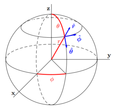
With \(V = V(r)\), the Schrödinger equation \(\eqref{eq:15}\) is separable in spherical coordinates. With reference to Fig. \(\PageIndex{1}\), the radial distance \(r\), polar angle \(\theta\) and azimuthal angle \(\phi\) are related to the usual cartesian coordinates by \[x=r\sin\theta\cos\phi ,\quad y=r\sin\theta\sin\phi ,\quad z=r\cos\theta ;\nonumber\] and by a change-of-coordinates calculation, the Laplacian can be shown to take the form \[\label{eq:17}\nabla^2=\frac{1}{r^2}\frac{\partial}{\partial r}\left(r^2\frac{\partial}{\partial r}\right)+\frac{1}{r^2\sin\theta}\frac{\partial}{\partial\theta}\left(\sin\theta\frac{\partial}{\partial\partial\theta}\right)+\frac{1}{r^2\sin^2\theta}\frac{\partial^2}{\partial\phi^2}.\]

The volume differential \(d\tau\) in spherical coordinates is given by \[\label{eq:18}d\tau =r^2\sin\theta drd\theta d\phi.\]

A complete solution to the hydrogen atom is somewhat involved, but nevertheless is such and important and fundamental problem that I will pursue it here. Our final result will lead us to obtain the three well-known quantum numbers of the hydrogen atom, namely the principle quantum number \(n\), the azimuthal quantum number \(l\), and the magnetic quantum number \(m\).

With \(\psi = \psi (r,\theta,\phi )\), we first separate out the angular dependence of the Schrödinger equation by writing \[\label{eq:19}\psi (r,\theta ,\phi)=R(r)Y(\theta , \phi ).\]

Substitution of \(\eqref{eq:19}\) into \(\eqref{eq:15}\) and using the spherical coordinate form for the Laplacian \(\eqref{eq:17}\) results in \[\begin{aligned}-\frac{\overline{h}^2}{2\mu}\left[\frac{Y}{r^2}\frac{d}{dr}\left(r^2\frac{dR}{dr}\right)+\frac{R}{r^2\sin\theta}\frac{\partial}{\partial\theta}\left(\sin\theta\frac{\partial Y}{\partial\theta}\right)\right.&\left.+\frac{R}{r^2\sin^2\theta}\frac{\partial^2Y}{\partial\phi^2}\right] \\ &+V(r)RY=ERY.\end{aligned}\]

To finish the separation step, we multiply by \(−2\mu r^2/\overline{h}^2RY\) and isolate the \(r\)-dependence on the left-hand side:

\[\frac{1}{R}\left[\frac{d}{dr}\left(r^2\frac{dR}{dr}\right)\right]+\frac{2\mu r^2}{\overline{h}^2}(E-V(r))=-\frac{1}{Y}\left[\frac{1}{\sin\theta}\frac{\partial}{\partial\theta}\left(\sin\theta\frac{\partial Y}{\partial\theta}\right)+\frac{1}{\sin^2\theta}\frac{\partial^2 Y}{\partial\phi^2}\right].\nonumber\]

The left-hand side is independent of \(\theta\) and \(\phi\) and the right-hand side is independent of \(r\), so that both sides equal a constant, which we will call \(\lambda_1\). The \(R\) equation is then obtained after multiplication by \(R/r^2\):

\[\label{eq:20}\frac{1}{r^2}\frac{d}{dr}\left(r^2\frac{dR}{dr}\right)+\left\{\frac{2\mu}{\overline{h}^2}[E-V(r)]-\frac{\lambda_1}{r^2}\right\}R=0.\]

The \(Y\) equation is obtained after multiplication by \(Y\):

\[\label{eq:21}\frac{1}{\sin\theta}\frac{\partial}{\partial\theta}\left(\sin\theta\frac{\partial Y}{\partial\theta}\right)+\frac{1}{\sin^2\theta}\frac{\partial^2Y}{\partial\phi^2}+\lambda_1Y=0.\]

To further separate the \(Y\) equation, we write \[\label{eq:22}Y(\theta, \phi)=\Theta(\theta)\Phi(\phi).\]

Substitution of \(\eqref{eq:22}\) into \(\eqref{eq:21}\) results in \[\frac{\Phi}{\sin\theta}\frac{d}{d\theta}\left(\sin\theta\frac{d\Theta}{d\theta}\right)+\frac{\Theta}{\sin^2\theta}\frac{d^2\Phi}{d\phi^2}+\lambda_1\Theta\Phi=0.\nonumber\]

To finish this separation, we multiply by \(\sin^2\theta/\Theta\Phi\) and isolate the \(\theta\)-dependence on the left-hand side to obtain \[\frac{\sin\theta}{\Theta}\frac{d}{d\theta}\left(\sin\theta\frac{d\Theta}{d\theta}\right)+\lambda_1\sin^2\theta=-\frac{1}{\Phi}\frac{d^2\Phi}{d\phi^2}.\nonumber\]

The left-hand side is independent of \(\phi\) and the right-hand side is independent of \(\theta\) so that both sides equal a constant, which we will call \(\lambda_2\). The \(\Theta\) equation is obtained after multiplication by \(\Theta /\sin^2\theta\):

\[\label{eq:23}\frac{1}{\sin\theta}\frac{d}{d\theta}\left(\sin\theta\frac{d\Theta}{d\theta}\right)+\left(\lambda_1-\frac{\lambda_2}{\sin^2\theta}\right)\Theta =0.\]

The \(\Phi\) equation is obtained after multiplication by \(\Phi\):

\[\label{eq:24}\frac{d^2\Phi}{d\phi^2}+\lambda_2\Phi=0.\]

The three eigenvalue ode equations for \(R(r),\: \Theta (\theta )\) and \(\Phi (\phi )\) are thus given by \(\eqref{eq:20}\), \(\eqref{eq:23}\) and \(\eqref{eq:24}\), with eigenvalues \(E\), \(\lambda_1\) and \(\lambda_2\).

Boundary conditions on the wavefunction determine the allowed values for the eigenvalues. We first solve \(\eqref{eq:24}\). The relevant boundary condition on \(\Phi = \Phi (\phi )\) is its single valuedness, and since the azimuthal angle is a periodic variable, we have \[\label{eq:25}\Phi (\phi +2\pi )=\Phi (\phi ).\]

Periodic solutions for \(\Phi (\phi )\) are possible only if \(\lambda_ 2 ≥ 0\). We therefore obtain using the complex form the general solutions of \(\eqref{eq:24}\):

\[\Phi (\phi)=\left\{\begin{array}{ll}Ae^{i\sqrt{\lambda_2}\phi}+Be^{-i\sqrt{\lambda_2}\phi},&\lambda_2=0, \\ C+D\phi ,&\lambda_2=0.\end{array}\right.\nonumber\]

The periodic boundary conditions given by \(\eqref{eq:25}\) requires that \(\sqrt{\lambda_2}\) is an integer and \(D = 0\). We therefore define \(\lambda_2 = m^2\), where \(m\) is any integer, and take as our eigenfunction \[\Phi_m(\phi)=\frac{1}{\sqrt{2\pi}}e^{im\phi},\nonumber\] where we have normalized \(\Phi_m\) so that \[\int_0^{2\pi}|\Phi_m(\phi)|^2d\phi =1.\nonumber\]

The quantum number \(m\) is commonly called the magnetic quantum number because when the atom is placed in an external magnetic field, its energy levels become dependent on \(m\).

To solve the \(\Theta\) equation \(\eqref{eq:23}\), we let \[w=\cos\theta ,P(w)=\Theta(\theta).\nonumber\]

Then \[\sin^2\theta=1-w^2\nonumber\] and \[\frac{d\Theta}{d\theta}=\frac{dP}{dw}\frac{dw}{d\theta}=-\sin\theta\frac{dP}{dw},\nonumber\] allowing us the replacement \[\frac{d}{d\theta}=-\sin\theta\frac{d}{dw}.\nonumber\]

With these substitutions and \(\lambda_2 = m^2\), \(\eqref{eq:23}\) becomes \[\label{eq:26}\frac{d}{dw}\left[(1-w^2)\frac{dP}{dw}\right]+\left(\lambda_1-\frac{m^2}{1-w^2}\right)P=0.\]

To solve \(\eqref{eq:26}\), we first consider the case \(m = 0\). Expanding the derivative, \(\eqref{eq:26}\) then becomes \[\label{eq:27}(1-w^2)\frac{d^2P}{dw}-2w\frac{dP}{dw}+\lambda_1P=0.\]

Since this is an ode with nonconstant coefficients, we try a power series ansatz of the usual form \[\label{eq:28}P(w)=\sum\limits_{k=0}^\infty a_kw^k.\]

Substitution of \(\eqref{eq:28}\) into \(\eqref{eq:27}\) yields \[\sum\limits_{k=2}^\infty k(k-1)a_kw^{k-2}-\sum\limits_{k=0}^\infty k(k-1)a_kw^k-\sum\limits_{k=0}^\infty 2ka_kw^k+\sum\limits_{k=0}^\infty\lambda_1a_kw^k=0.\nonumber\]

Shifting the index in the first expression and combining terms results in \[\sum\limits_{k=0}^\infty\left\{ (k+2)(k+1)a_{k+2}-[(k(k+1)-\lambda_1]a_k\right\}w^k=0.\nonumber\]

Finally, setting the coefficients of the power series equal to zero results in the recursion relation \[a_{k+2}=\frac{k(k+1)-\lambda_1}{(k+2)(k+1)}a_k.\nonumber\]

Even and odd coefficients decouple, and the even solution is of the form \[P_{\text{even}}(w)=\sum\limits_{n=0}^\infty a_{2n}w^{2n},\nonumber\] and the odd solution is of the form \[P_{\text{odd}}(w)=\sum\limits_{n=0}^\infty a_{2n+1}w^{2n+1}.\nonumber\]

An application of Gauss’s test for series convergence can show that both the even and the odd solutions diverge when \(|w| = 1\) unless the series terminates. Since the wavefunction must be everywhere finite, the series must terminate and we obtain the discrete eigenvalues \[\label{eq:29}\lambda_1=l(l+1),\quad\text{for }l=0,1,2,\ldots .\]

The quantum number \(l\) is commonly called the azimuthal quantum number despite having arisen from the polar angle equation. The resulting eigenfunctions \(P_l(w)\) are called the Legendre polynomials. These polynomials are usually normalized such that \(P_l(1) = 1\), and the first four Legendre polynomials are given by \[\begin{array}{ll}P_0(w)=1,&P_1(w)=w, \\ P_2(w)=\frac{1}{2}(3w^2-1), &P_3(w)=\frac{1}{2}(5w^3-3w).\end{array}\nonumber\]

With \(\lambda_1 = l(l + 1)\), we now reconsider \(\eqref{eq:26}\). Expanding the derivative gives \[\label{eq:30}(1-w^2)\frac{d^2P}{dw^2}-2w\frac{dP}{dw}+\left( l(l+1)-\frac{m^2}{1-w^2}\right)P=0.\]

Equation \(\eqref{eq:30}\) is called the associated Legendre equation. The associated Legendre equation with \(m = 0\), \[\label{eq:31}(1-w^2)\frac{d^2P}{dw^2}-2w\frac{dP}{dw}+l(l+1)P=0,\] is called the Legendre equation. We now know that the Legendre equation has eigenfunctions given by the Legendre polynomials, \(P_l (w)\). Amazingly, the eigenfunctions of the associated Legendre equation can be obtained directly from the Legendre polynomials. For ease of notation, we will assume that \(m > 0\). To include the cases \(m < 0\), we need only replace \(m\) everywhere by \(|m|\).

To see how to obtain the eigenfunctions of the associated Legendre equation, we will first show how to derive the associated Legendre equation from the Legendre equation. We will need to differentiate the Legendre equation \(\eqref{eq:31}\) \(m\) times and to do this we will make use of Leibnitz’s formula for the \(m\)th derivative of a product:

\[\frac{d^m}{dx^m}[f(x)g(x)]=\sum\limits_{j=0}^m\left(\begin{array}{c}m\\j\end{array}\right)\frac{d^jf}{dx^j}\frac{d^{m-j}g}{dx^{m-j}},\nonumber\] where the binomial coefficients are given by \[\left(\begin{array}{c}m\\j\end{array}\right)=\frac{m!}{j!(m-j)!}.\nonumber\]

We first compute \[\frac{d^m}{dw^m}\left[(1-w^2)\frac{d^2P}{dw^2}\right]=\sum\limits_{j=0}^m\left(\begin{array}{c}m\\j\end{array}\right)\left[\frac{d^j}{dw^j}(1-w^2)\right]\left[\frac{d^{m-j}}{dw^{m-j}}\frac{d^2P}{dw^2}\right].\nonumber\]

Only the terms \(j = 0,\: 1\) and \(2\) contribute, and using \[\left(\begin{array}{c}m\\0\end{array}\right)=1,\quad\left(\begin{array}{c}m\\1\end{array}\right)=m,\quad\left(\begin{array}{c}m\\2\end{array}\right)=\frac{m(m-1)}{2},\nonumber\] and the more compact notation \[\label{eq:32}\frac{d^nP}{dw^n}=P^{(n)}(w),\nonumber\] we find \[\frac{d^m}{dw^m}\left[(1-w^2)P^{(2)}\right]=(1-w^2)P^{(m+2)}-2mwP^{(m+1)}-m(m-1)P^{(m)}.\]

We next compute \[\frac{d^m}{dw^m}\left[2w\frac{dP}{dw}\right]=\sum\limits_{j=0}^m\left(\begin{array}{c}m\\j\end{array}\right)\left[\frac{d^j}{2w^j}2w\right]\left[\frac{d^{m-j}}{dw^{m-j}}\frac{dP}{dw}\right].\nonumber\]

Here, only the terms \(j = 0\) and \(1\) contribute, and we find \[\label{eq:33}\frac{d^m}{dw^m}\left[2wP^{(1)}\right]=2wP^{(m+1)}+2mP^{(m)}.\]

Differentiating the Legendre equation \(\eqref{eq:31}\) \(m\) times, using \(\eqref{eq:32}\) and \(\eqref{eq:33}\), and defining \[p(w)=P^{(m)}(w)\nonumber\] results in \[\label{eq:34}(1-w^2)\frac{d^2P}{dw^2}-2(1+m)w\frac{dp}{dw}+[l(l+1)-m(m+1)]p=0.\]

Finally, we define \[\label{eq:35}q(w)=(1-w^2)^{m/2}p(w).\]

Then using \[\label{eq:36}\frac{dp}{dw}=(1-w^2)^{-m/2}\left(\frac{dq}{dw}+\frac{mwq}{1-w^2}\right)\] and \[\label{eq:37}\frac{d^2p}{dw^2}=(1-w^2)^{-m/2}\left\{\frac{d^2q}{dw^2}+\frac{2mw}{1-w^2}\frac{dq}{dw}+\left[\frac{m(m+2)w^2}{(1-w^2)^2}+\frac{m}{1-w^2}\right]q\right\},\] we substitute \(\eqref{eq:36}\) and \(\eqref{eq:37}\) into \(\eqref{eq:34}\) and cancel the common factor of \((1 − w^2)^{−m/2}\) to obtain \[(1-w^2)\frac{d^2q}{dw^2}-2w\frac{dq}{dw}+\left[l(l+1)-\frac{m^2}{1-w^2}\right]q=0,\nonumber\] which is just the associated Legendre equation \(\eqref{eq:30}\) for \(q = q(w)\). We may call the eigenfunctions of the associated Legendre equation \(P_{lm}(w)\), and with \(q(w) = P_{lm}(w)\), we have determined the following relationship between the eigenfunctions of the associated Legendre equation and the Legendre polynomials:

\[\label{eq:38}P_{lm}(w)=(1-w^2)^{|m|/2}\frac{d^{|m|}}{dw^{|m|}}P_l(w),\] where we have now replaced \(m\) by its absolute value to include the possibility of negative integers. Since \(P_l(w)\) is a polynomial of order \(l\), the expression given by \(\eqref{eq:38}\) is nonzero only when \(|m| ≤ l\). Sometimes the magnetic quantum number \(m\) is written as \(m_l\) to signify that its range of allowed values depends on the value of \(l\).

At last, we need to solve the eigenvalue ode for \(R = R(r)\) given by \(\eqref{eq:20}\), with \(V(r)\) given by \(\eqref{eq:16}\) and \(\lambda_1\) given by \(\eqref{eq:29}\). The radial equation is now \[\label{eq:39}\frac{1}{r^2}\frac{d}{dr}\left(r^2\frac{dR}{dr}\right)+\left\{\frac{2\mu}{\overline{h}^2}\left[E+\frac{Ze^2}{4\pi\epsilon_0r}\right]-\frac{l(l+1)}{r^2}\right\}R=0.\]

Note that each term in this equation has units of one over length squared times \(R\) and that \(E < 0\) for a bound state solution.

It is customary to nondimensionalize the length scale so that \(2\mu E/\overline{h}^2 = −1/4\) in dimensionless units. Furthermore, multiplication of \(R(r)\) by \(r\) can also simplify the derivative term. To these ends, we change variables to \[\rho=\frac{\sqrt{8\mu |E|}}{\overline{h}}r,\quad u(\rho )=rR(r),\nonumber\] and obtain after multiplication of the entire equation by \(\rho\) the simplified equation \[\label{eq:40}\frac{d^2u}{d\rho^2}+\left\{\frac{\alpha}{\rho}-\frac{1}{4}-\frac{l(l+1)}{\rho^2}\right\}u=0,\] where \(\alpha\) now plays the role of a dimensionless eigenvalue, and is given by \[\label{eq:41}\alpha=\frac{Ze^2}{4\pi\epsilon_0\overline{h}}\sqrt{\frac{\mu}{2|E|}}.\]

As we saw for the problem of the simple harmonic oscillator, it may be helpful to consider the behavior of \(u = u(\rho )\) for large \(\rho\). For large \(\rho\), \(\eqref{eq:40}\) simplifies to \[\frac{d^2u}{d\rho^2}-\frac{1}{4}u=0,\nonumber\] with two independent solutions \[u(\rho)=\left\{\begin{array}{l}e^{\rho /2}, \\ e^{-\rho /2}.\end{array}\right.\nonumber\]

Since the relevant boundary condition here must be \(\lim_{\rho\to\infty} u(\rho ) = 0\), only the second decaying exponential solution can be allowed.

We can also consider the behavior of \(\eqref{eq:40}\) for small \(\rho\). Multiplying by \(\rho^2\), and neglecting terms proportional to \(\rho\) and \(\rho^2\) that are not balanced by derivatives, results in the Cauchy-Euler equation \[\rho^2\frac{d^2u}{d\rho^2}-l(l+u)=0,\nonumber\] which can be solved by the ansatz \(u = \rho^s\). After canceling \(\rho^s\), we obtain \[s(s − 1) − l(l + 1) = 0,\nonumber\] which has the two solutions \[s=\left\{\begin{array}{l}l+1, \\ -l.\end{array}\right.\nonumber\]

If \(R = R(r)\) is finite at \(r = 0\), the relevant boundary condition here must be \(\lim_{\rho\to 0} u(\rho ) = 0\) so that only the first solution \(u(\rho ) \sim \rho^{l+1}\) can be allowed.

Combining these asymptotic results for large and small \(\rho\), we now try to substitute \[\label{eq:42}u(\rho)=\rho^{l+1}e^{-\rho /2}F(\rho )\] into \(\eqref{eq:40}\). After some algebra, the resulting differential equation for \(F = F(\rho )\) is found to be \[\frac{d^2F}{d\rho^2}+\left(\frac{2(l+1)}{\rho}-1\right)\frac{dF}{d\rho}+\frac{\alpha -(l+1)}{\rho}F=0.\nonumber\]

We are now in a position to try a power-series ansatz of the form \[F(\rho)=\sum\limits_{k=0}^\infty a_k\rho^k\nonumber\] to obtain \[\sum\limits_{k=2}^\infty k(k-1)a_k\rho^{k-2}+\sum\limits_{k=1}^\infty 2(l+1)ka_k\rho^{k-2}-\sum\limits_{k=1}^\infty ka_k\rho^{k-1}+\sum\limits_{k=0}^\infty [\alpha -(l+1_]a_k\rho^{k-1}=0.\nonumber\]

Shifting indices, bringing the lower summations down to zero by including zero terms, and finally combining terms, we obtain \[\sum\limits_{k=0}^\infty\left\{[(k+1)(k+2(l+1))]a_{k+1}-(1+l+k-\alpha )a_k\right\}\rho^{k-1}=0.\nonumber\]

Setting the coefficients of this power series equal to zero gives us the recursion relation \[a_{k+1}=\frac{1+l+k-\alpha}{(k+1)(k+2(l+1))}a_k.\nonumber\]

For large \(k\), we have \(a_{k+1}/a_k\to 1/k\), which has the same behavior as the power series for \(e^\rho\), resulting in a solution for \(u = u(\rho )\) that behaves as \(u(\rho ) = e^{\rho /2}\) for large \(\rho\). To exclude this solution, we must require the power series to terminate, and we obtain the discrete eigenvalues \[\alpha =1+l+n',\quad n'=0,1,2,\ldots .\nonumber\]

The function \(F = F(\rho )\) is then a polynomial of degree \(n'\) and is known as an associated Laguerre polynomial.

The energy levels of the hydrogen-like atoms are determined from the allowed \(\alpha\) eigenvalues. Using \(\eqref{eq:41}\), and defining \[n=1+l+n',\nonumber\] for the nonnegative integer values of \(n'\) and \(l\), we have \[E_n=-\frac{\mu Z^2e^4}{2(4\pi\epsilon_0)^2\overline{h}^2n^2},\quad n=1,2,3,\ldots .\nonumber\]

If we consider a specific energy level \(E_n\), then the allowed values of the quantum number \(l\) are nonnegative and satisfy \(l = n − n' − 1\). For fixed \(n\) then, the quantum number \(l\) can range from \(0\) (when \(n' = n − 1\)) to \(n − 1\) (when \(n' = 0\)).

To summarize, there are three integer quantum numbers \(n,\: l,\) and \(m\), with \[\begin{aligned}n&=1,2,3,\ldots , \\ l&=0,1,\ldots ,n-1, \\ m&=-l,\ldots ,l,\end{aligned}\] and for each choice of quantum numbers \((n, l, m)\) there is a corresponding energy eigenvalue \(E_n\), which depends only on \(n\), and a corresponding energy eigenfunction \(\psi = \psi_{nlm}(r, \theta , \phi )\), which depends on all three quantum numbers.

For illustration, we exhibit the wavefunctions of the ground state and the first excited states of hydrogen-like atoms. Making use of the volume differential \(\eqref{eq:18}\), normalization is such that \[\int_0^\infty \int_0^\pi \int_0^{2\pi} |\psi_{nlm}(r,\theta ,\phi )|^2r^2\sin\theta dr\:d\theta\:d\phi =1.\nonumber\]

Using the definition of the Bohr radius as \[a_0=\frac{4\pi\epsilon _0\overline{h}^2}{\mu e^2},\nonumber\] the ground state wavefunction is given by \[\psi_{100}=\frac{1}{\sqrt{\pi}}\left(\frac{Z}{a_0}\right)^{3/2}e^{-Zr/a_0},\nonumber\] and the three degenerate first excited states are given by \[\begin{aligned} \psi_{200}& =\frac{1}{4\sqrt{2\pi}}\left(\frac{Z}{a_0}\right)^{3/2}\left(2-\frac{Zr}{a_0}\right)e^{-Zr/2a_0}, \\ \psi_{210}&=\frac{1}{4\sqrt{2\pi}}\left(\frac{Z}{a_0}\right)^{3/2}\frac{Zr}{a_0}e^{-Zr/2a_0}\cos\theta , \\ \psi_{21\pm 1}&=\frac{1}{8\sqrt{\pi}}\left(\frac{Z}{a_0}\right)^{3/2}\frac{Zr}{a_0}e^{-Zr/2a_0}\sin\theta e^{\pm i\phi}.\end{aligned}\]