10.1: Introduction to Cartesian Coordinates in Space

Up to this point in this text we have considered mathematics in a 2--dimensional world. We have plotted graphs on the \(x\)-\(y\) plane using rectangular and polar coordinates and found the area of regions in the plane. We have considered properties of solid objects, such as volume and surface area, but only by first defining a curve in the plane and then rotating it out of the plane.

While there is wonderful mathematics to explore in "2D,'' we live in a "3D'' world and eventually we will want to apply mathematics involving this third dimension. In this section we introduce Cartesian coordinates in space and explore basic surfaces. This will lay a foundation for much of what we do in the remainder of the text.

Each point \(P\) in space can be represented with an ordered triple, \(P=(a,b,c)\), where \(a\), \(b\) and \(c\) represent the relative position of \(P\) along the \(x\)-, \(y\)- and \(z\)-axes, respectively. Each axis is perpendicular to the other two.

Visualizing points in space on paper can be problematic, as we are trying to represent a 3-dimensional concept on a 2--dimensional medium. We cannot draw three lines representing the three axes in which each line is perpendicular to the other two. Despite this issue, standard conventions exist for plotting shapes in space that we will discuss that are more than adequate.

One convention is that the axes must conform to the right hand rule. This rule states that when the index finger of the right hand is extended in the direction of the positive \(x\)-axis, and the middle finger (bent "inward'' so it is perpendicular to the palm) points along the positive \(y\)-axis, then the extended thumb will point in the direction of the positive \(z\)-axis. (It may take some thought to verify this, but this system is inherently different from the one created by using the "left hand rule.''). There are two popular methods to draw axes that we briefly discuss.

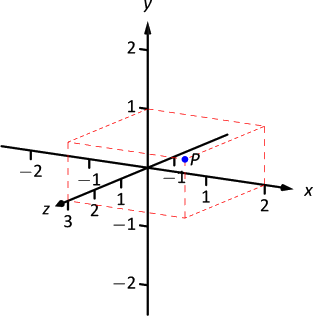
In Figure \(\PageIndex{1}\) we see the point \(P=(2,1,3)\) plotted on a set of axes. The basic convention here is that the \(x\)-\(y\) plane is drawn in its standard way, with the \(z\)-axis down to the left. The perspective is that the paper represents the \(x\)-\(y\) plane and the positive \(z\) axis is coming up, off the page. This method is preferred by many engineers. Because it can be hard to tell where a single point lies in relation to all the axes, dashed lines have been added to let one see how far along each axis the point lies.

Figure \(\PageIndex{1}\): Plotting the point \(P=(2,1,3)\) in space.

One can also consider the \(x\)-\(y\) plane as being a horizontal plane in, say, a room, where the positive \(z\)-axis is pointing up. When one steps back and looks at this room, one might draw the axes as shown in Figure \(\PageIndex{2}\). The same point \(P\) is drawn, again with dashed lines. This point of view is preferred by most mathematicians, and is the convention adopted by this text.

Figure \(\PageIndex{2}\): Plotting the point \(P=(2,1,3)\) in space with a perspective used in this text.

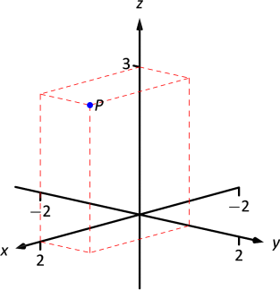
Note

As long as the coordinate axes are positioned so that they follow the right hand rule, it does not matter how the axes are drawn on paper.

Measuring Distances

It is of critical importance to know how to measure distances between points in space. The formula for doing so is based on measuring distance in the plane, and is known (in both contexts) as the Euclidean measure of distance.

Definition 48: distance in space

Let \(P=(x_1,y_1,z_1)\) and \(Q = (x_2,y_2,z_2)\) be points in space. The distance \(D\) between \(P\) and \(Q\) is

\[D = \sqrt{(x_2-x_1)^2+(y_2-y_1)^2+(z_2-z_1)^2}.\]

We refer to the line segment that connects points \(P\) and \(Q\) in space as \(\overline{PQ}\), and refer to the length of this segment as \(||\overline{PQ}||\). The above distance formula allows us to compute the length of this segment.

Example \(\PageIndex{1}\): Length of a line segment

Let \(P = (1,4,-1)\) and let \(Q = (2,1,1)\). Draw the line segment \(\overline{PQ}\) and find its length.

Solution

The points \(P\) and \(Q\) are plotted in Figure \(\PageIndex{3}\); no special consideration need be made to draw the line segment connecting these two points; simply connect them with a straight line.

Figure \(\PageIndex{3}\): Plotting points \(P\) and \(Q\) in Example \(\PageIndex{1}\).

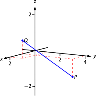
One cannot actually measure this line on the page and deduce anything meaningful; its true length must be measured analytically. Applying Definition 48, we have

\[||\overline{PQ}|| = \sqrt{(2-1)^2+(1-4)^2+(1-(-1))^2} = \sqrt{14}\approx 3.74.\]

Spheres

Just as a circle is the set of all points in the plane equidistant from a given point (its center), a sphere is the set of all points in space that are equidistant from a given point. Definition 48 allows us to write an equation of the sphere. We start with a point \(C = (a,b,c)\) which is to be the center of a sphere with radius \(r\). If a point \(P=(x,y,z)\) lies on the sphere, then \(P\) is \(r\) units from \(C\); that is,

\[||\overline{PC}|| = \sqrt{(x-a)^2+(y-b)^2+(z-c)^2} = r.\]

Squaring both sides, we get the standard equation of a sphere in space with center at \(C=(a,b,c)\) with radius \(r\), as given in the following Key Idea.

KEY IDEA 45: STANDARD EQUATION OF A SPHERE IN SPACE

The standard equation of the sphere with radius \(r\), centered at \(C=(a,b,c)\), is \[(x-a)^2+(y-b)^2+(z-c)^2=r^2.\]

Example \(\PageIndex{2}\): Equation of a sphere

Find the center and radius of the sphere defined by \(x^2+2x+y^2-4y+z^2-6z=2.\)

Solution

To determine the center and radius, we must put the equation in standard form. This requires us to complete the square (three times).

\[\begin{align*}
x^2+2x+y^2-4y+z^2-6z&=2 \\
(x^2+2x+1) + (y^2-4y+4)+ (z^2-6z+9) - 14 &= 2\\
(x+1)^2 + (y-2)^2 + (z-3)^2 &= 16
\end{align*}\]

The sphere is centered at \((-1,2,3)\) and has a radius of 4.

The equation of a sphere is an example of an implicit function defining a surface in space. In the case of a sphere, the variables \(x\), \(y\) and \(z\) are all used. We now consider situations where surfaces are defined where one or two of these variables are absent.

Introduction to Planes in Space

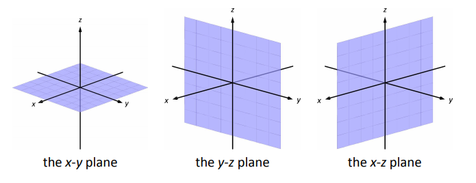
The coordinate axes naturally define three planes (shown in Figure \(\PageIndex{4}\)), the coordinate planes: the \(x\)-\(y\) plane, the \(y\)-\(z\) plane and the \(x\)-\(z\) plane. The \(x\)-\(y\) plane is characterized as the set of all points in space where the \(z\)-value is 0. This, in fact, gives us an equation that describes this plane: \(z=0\). Likewise, the \(x\)-\(z\) plane is all points where the \(y\)-value is 0, characterized by \(y=0\).

Figure \(\PageIndex{4}\): The coordinate planes.

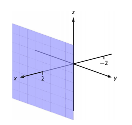
The equation \(x=2\) describes all points in space where the \(x\)-value is 2. This is a plane, parallel to the \(y\)-\(z\) coordinate plane, shown in Figure \(\PageIndex{5}\).

Figure \(\PageIndex{5}\): The plane \(x=2\).

Example \(\PageIndex{3}\): Regions defined by planes

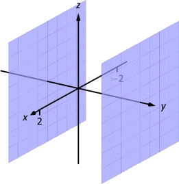
Sketch the region defined by the inequalities \(-1\leq y\leq 2\).

Solution

The region is all points between the planes \(y=-1\) and \(y=2\). These planes are sketched in Figure \(\PageIndex{6}\), which are parallel to the \(x\)-\(z\) plane. Thus the region extends infinitely in the \(x\) and \(z\) directions, and is bounded by planes in the \(y\) direction.

Figure \(\PageIndex{6}\): Sketching the boundaries of a region in Example \(\PageIndex{3}\).

Cylinders

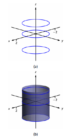
The equation \(x=1\) obviously lacks the \(y\) and \(z\) variables, meaning it defines points where the \(y\) and \(z\) coordinates can take on any value. Now consider the equation \(x^2+y^2=1\) in space. In the plane, this equation describes a circle of radius 1, centered at the origin. In space, the \(z\) coordinate is not specified, meaning it can take on any value. In Figure \(\PageIndex{7a}\), we show part of the graph of the equation \(x^2+y^2=1\) by sketching 3 circles: the bottom one has a constant \(z\)-value of \(-1.5\), the middle one has a \(z\)-value of 0 and the top circle has a \(z\)-value of 1. By plotting all possible \(z\)-values, we get the surface shown in Figure \(\PageIndex{7b}\).
This surface looks like a "tube,'' or a "cylinder''; mathematicians call this surface a cylinder for an entirely different reason.

Figure \(\PageIndex{7}\): Sketching \(x^2+y^2=1\).

Definition 49: CYLINDER, Directrix and Rulings

Let \(C\) be a curve in a plane and let \(L\) be a line not parallel to \(C\). A cylinder is the set of all lines parallel to \(L\) that pass through \(C\). The curve \(C\) is the directrix of the cylinder, and the lines are the rulings.

In this text, we consider curves \(C\) that lie in planes parallel to one of the coordinate planes, and lines \(L\) that are perpendicular to these planes, forming right cylinders. Thus the directrix can be defined using equations involving 2 variables, and the rulings will be parallel to the axis of the 3\(^\text{rd}\) variable.

In the example preceding the definition, the curve \(x^2+y^2=1\) in the \(x\)-\(y\) plane is the directrix and the rulings are lines parallel to the \(z\)-axis. (Any circle shown in Figure 10.8 can be considered a directrix; we simply choose the one where \(z=0\).) Sample rulings can also be viewed in part (b) of the figure. More examples will help us understand this definition.

Example \(\PageIndex{4}\): Graphing cylinders

Graph the cylinder following cylinders.

1. \(z=y^2\)
2. \(x=\sin z\)

Solution

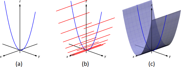
1. We can view the equation \(z=y^2\) as a parabola in the \(y\)-\(z\) plane, as illustrated in Figure \(\PageIndex{8a}\). As \(x\) does not appear in the equation, the rulings are lines through this parabola parallel to the \(x\)-axis, shown in Figure \(\PageIndex{8b}\). These rulings give a general idea as to what the surface looks like, drawn in (c).

Figure \(\PageIndex{8}\): Sketching the cylinder defined by \(z=y^2\).

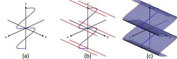
2. We can view the equation \(x=\sin z\) as a sine curve that exists in the \(x\)-\(z\) plane, as shown in Figure \(\PageIndex{9a}\). The rules are parallel to the \(y\) axis as the variable \(y\) does not appear in the equation \(x=\sin z\); some of these are shown in Figure \(\PageIndex{9b}\). The surface is shown in part (c) of the figure.

Figure \(\PageIndex{9}\): Sketching the cylinder defined by \(x=\sin z\).

Surfaces of Revolution

One of the applications of integration we learned previously was to find the volume of solids of revolution -- solids formed by revolving a curve about a horizontal or vertical axis. We now consider how to find the equation of the surface of such a solid.

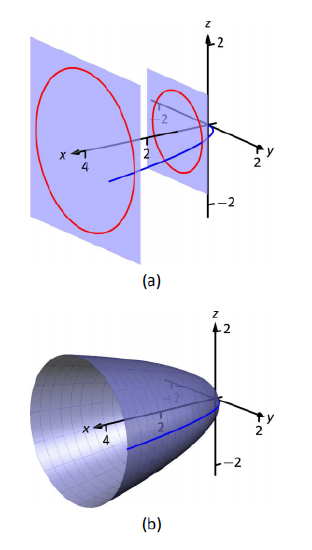
Consider the surface formed by revolving \(y=\sqrt{x}\) about the \(x\)-axis. Cross--sections of this surface parallel to the \(y\)-\(z\) plane are circles, as shown in Figure \(\PageIndex{1a}\). Each circle has equation of the form \(y^2+z^2=r^2\) for some radius \(r\). The radius is a function of \(x\); in fact, it is \(r(x) = \sqrt{x}\). Thus the equation of the surface shown in Figure \(\PageIndex{10b}\) is \(y^2+z^2=(\sqrt{x})^2.\)

Figure \(\PageIndex{10}\): Introducing surfaces of revolution.

We generalize the above principles to give the equations of surfaces formed by revolving curves about the coordinate axes.

KEY IDEA 46: SURFACES OF REVOLUTION, PART 1

Let \(r\) be a radius function.

1. The equation of the surface formed by revolving \(y=r(x)\) or \(z=r(x)\) about the \(x\)-axis is \(y^2+z^2=r(x)^2\).
2. The equation of the surface formed by revolving \(x=r(y)\) or \(z=r(y)\) about the \(y\)-axis is \(x^2+z^2=r(y)^2\).
3. The equation of the surface formed by revolving \(x=r(z)\) or \(y=r(z)\) about the \(z\)-axis is \(x^2+y^2=r(z)^2\).

Example \(\PageIndex{5}\): Finding equation of a surface of revolution

Let \(y=\sin z\) on \([0,\pi]\). Find the equation of the surface of revolution formed by revolving \(y=\sin z\) about the \(z\)-axis.

Solution

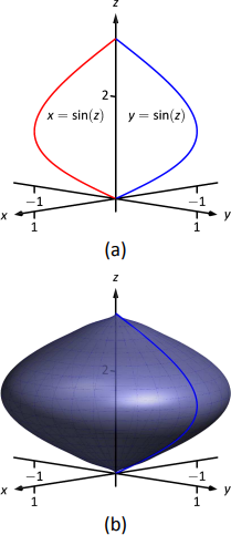
Using Key Idea 46, we find the surface has equation \(x^2+y^2=\sin^2z\). The curve is sketched in Figure \(\PageIndex{11a}\) and the surface is drawn in Figure \(\PageIndex{11b}\).

Note how the surface (and hence the resulting equation) is the same if we began with the curve \(x=\sin z\), which is also drawn in Figure \(\PageIndex{11a}\).

Figure \(\PageIndex{11}\): Revolving \(y=\sin z\) about the z-axis in Example \(\PageIndex{5}\).

This particular method of creating surfaces of revolution is limited. For instance, in Section 7.3 we found the volume of the solid formed by revolving \(y=\sin x\) about the \(y\)-axis. Our current method of forming surfaces can only rotate \(y=\sin x\) about the \(x\)-axis. Trying to rewrite \(y=\sin x\) as a function of \(y\) is not trivial, as simply writing \(x=\sin^{-1}y\) only gives part of the region we desire.

What we desire is a way of writing the surface of revolution formed by rotating \(y=f(x)\) about the \(y\)-axis. We start by first recognizing this surface is the same as revolving \(z=f(x)\) about the \(z\)-axis. This will give us a more natural way of viewing the surface.

A value of \(x\) is a measurement of distance from the \(z\)-axis. At the distance \(r\), we plot a \(z\)-height of \(f(r)\). When rotating \(f(x)\) about the \(z\)-axis, we want all points a distance of \(r\) from the \(z\)-axis in the \(x\)-\(y\) plane to have a \(z\)-height of \(f(r)\). All such points satisfy the equation \(r^2=x^2+y^2\); hence \(r=\sqrt{x^2+y^2}\). Replacing \(r\) with \(\sqrt{x^2+y^2}\) in \(f(r)\) gives \(z=f(\sqrt{x^2+y^2})\). This is the equation of the surface.

KEY IDEA 47: SURFACES OF REVOLUTION, PART 2

Let \(z=f(x)\), \(x\geq 0\), be a curve in the \(x\)-\(z\) plane. The surface formed by revolving this curve about the \(z\)-axis has equation \(z=f \left(\sqrt{x^2+y^2} \right)\).

Example \(\PageIndex{6}\): Finding equation of surface of revolution

Find the equation of the surface found by revolving \(z=\sin x\) about the \(z\)-axis.

Solution

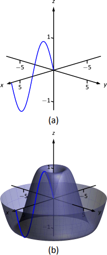
Using Key Idea 47, the surface has equation \(z=\sin \left(\sqrt{x^2+y^2} \right)\). The curve and surface are graphed in Figure \(\PageIndex{12}\).

Figure \(\PageIndex{12}\): Revolving \(z=\sin x\) about the z-axis in Example \(\PageIndex{6}\).

Quadric Surfaces

Spheres, planes and cylinders are important surfaces to understand. We now consider one last type of surface, a quadric surface. The definition may look intimidating, but we will show how to analyze these surfaces in an illuminating way.

Definition 50: QUADRIC SURFACE

A quadric surface is the graph of the general second--degree equation in three variables:

\[Ax^2+By^2+Cz^2+Dxy+Exz+Fyz+Gx+Hy+Iz+J=0.\]

When the coefficients \(D\), \(E\) or \(F\) are not zero, the basic shapes of the quadric surfaces are rotated in space. We will focus on quadric surfaces where these coeffiecients are 0; we will not consider rotations. There are six basic quadric surfaces: the elliptic paraboloid, elliptic cone, ellipsoid, hyperboloid of one sheet, hyperboloid of two sheets, and the hyperbolic paraboloid.

We study each shape by considering traces, that is, intersections of each surface with a plane parallel to a coordinate plane. For instance, consider the elliptic paraboloid \(z= x^2/4+y^2\), shown in Figure 10.13. If we intersect this shape with the plane \(z=d\) (i.e., replace \(z\) with \(d\)), we have the equation:

\[d = \frac{x^2}4+y^2.\]

Divide both sides by \(d\):

\[1 = \frac{x^2}{4d} + \frac{y^2}{d}.\]

This describes an ellipse -- so cross sections parallel to the \(x\)-\(y\) coordinate plane are ellipses. This ellipse is drawn in Figure \(\PageIndex{13}\).

Figure \(\PageIndex{13}\): The elliptic paraboloid \(z=x^2/4+y^2\).

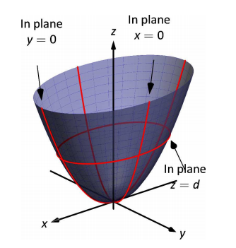
Now consider cross sections parallel to the \(x\)-\(z\) plane. For instance, letting \(y=0\) gives the equation \(z=x^2/4\), clearly a parabola. Intersecting with the plane \(x=0\) gives a cross section defined by \(z=y^2\), another parabola. These parabolas are also sketched in the figure.

Thus we see where the elliptic paraboloid gets its name: some cross sections are ellipses, and others are parabolas.

Such an analysis can be made with each of the quadric surfaces. We give a sample equation of each, provide a sketch with representative traces, and describe these traces.

Elliptic Paraboloid, \(z=\frac{x^2}{a^2}+\frac{y^2}{b^2}\)

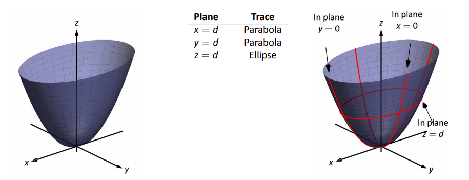
One variable in the equation of the elliptic paraboloid will be raised to the first power; above, this is the \(z\) variable. The paraboloid will "open'' in the direction of this variable's axis. Thus \(x= y^2/a^2+z^2/b^2\) is an elliptic paraboloid that opens along the \(x\)-axis.

Multiplying the right hand side by \((-1)\) defines an elliptic paraboloid that "opens'' in the opposite direction.

Elliptic Cone, \( z^2=\frac{x^2}{a^2}+\frac{y^2}{b^2}\)

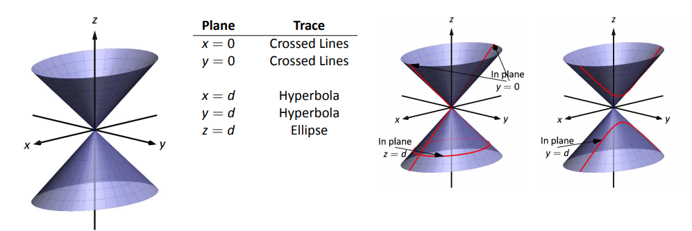
One can rewrite the equation as \(z^2-x^2/a^2-y^2/{b^2} = 0\). The one variable with a positive coefficient corresponds to the axis that the cones "open'' along.

Ellipsoid, \( \frac{x^2}{a^2}+\frac{y^2}{b^2}+\frac{z^2}{c^2}=1\)

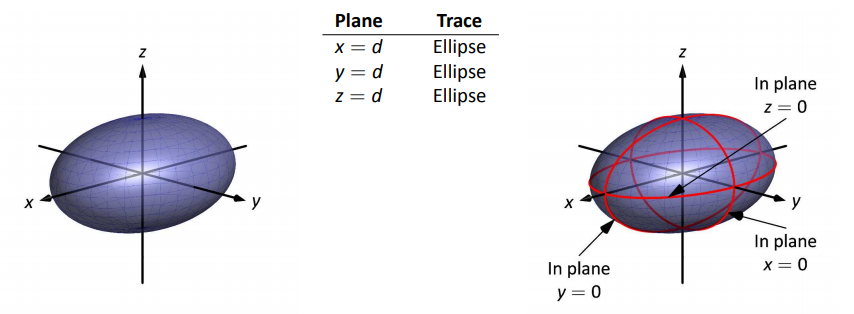
If \(a=b=c\neq0\), the ellipsoid is a sphere with radius \(a\); compare to Key Idea 45.

Hyperboloid of One Sheet, \(\frac{x^2}{a^2}+\frac{y^2}{b^2}-\frac{z^2}{c^2}=1\)

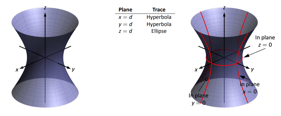
The one variable with a negative coefficient corresponds to the axis that the hyperboloid "opens'' along.

Hyperboloid of Two Sheets, \( \frac{z^2}{c^2}-\frac{x^2}{a^2}-\frac{y^2}{b^2}=1\)

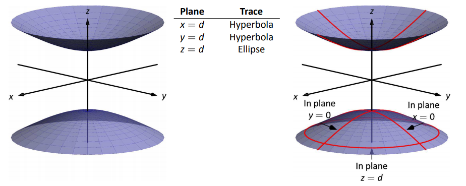
The one variable with a positive coefficient corresponds to the axis that the hyperboloid "opens'' along. In the case illustrated, when \(|d|<|c|\), there is no trace.

Hyperbolic Paraboloid, \( z=\frac{x^2}{a^2}-\frac{y^2}{b^2}\)

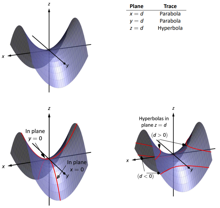
The parabolic traces will open along the axis of the one variable that is raised to the first power.

Example \(\PageIndex{7}\): Sketching quadric surfaces

Sketch the quadric surface defined by the given equation.

1. \(y=\frac{x^2}{4}+\frac{z^2}{16}\)
2. \( x^2+\frac{y^2}{9}+\frac{z^2}{4}=1.\)
3. \( z=y^2-x^2\).

Solution

1. \( y=\frac{x^2}{4}+\frac{z^2}{16}\):
   
   We first identify the quadric by pattern--matching with the equations given previously. Only two surfaces have equations where one variable is raised to the first power, the elliptic paraboloid and the hyperbolic paraboloid. In the latter case, the other variables have different signs, so we conclude that this describes a hyperbolic paraboloid. As the variable with the first power is \(y\), we note the paraboloid opens along the \(y\)-axis.
   
   To make a decent sketch by hand, we need only draw a few traces. In this case, the traces \(x=0\) and \(z=0\) form parabolas that outline the shape.
   
   \(x=0\): The trace is the parabola \(y=z^2/16\)
   
   \(z=0\): The trace is the parabola \(y=x^2/4\).
   
   Graphing each trace in the respective plane creates a sketch as shown in Figure \(\PageIndex{14a}\). This is enough to give an idea of what the paraboloid looks like. The surface is filled in in Figure \(\PageIndex{14b}\).

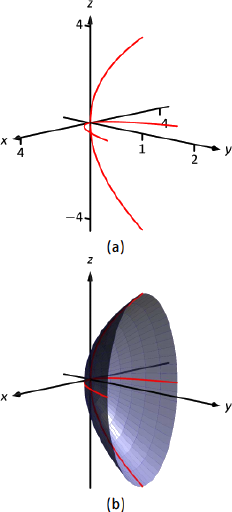
Figure \(\PageIndex{14}\): Sketching an elliptic paraboloid.

2. \( x^2+\frac{y^2}{9}+\frac{z^2}{4}=1:\)
   
   This is an ellipsoid. We can get a good idea of its shape by drawing the traces in the coordinate planes.
   
   \(x=0\): The trace is the ellipse \(\frac{y^2}{9}+\frac{z^2}{4}=1\). The major axis is along the \(y\)--axis with length 6 (as \(b=3\), the length of the axis is 6); the minor axis is along the \(z\)-axis with length 4.
   
   \(y=0\): The trace is the ellipse \( x^2+\frac{z^2}{4}=1.\) The major axis is along the \(z\)-axis, and the minor axis has length 2 along the \(x\)-axis.
   
   \(z=0\): The trace is the ellipse \( x^2+\frac{y^2}{9}=1,\) with major axis along the \(y\)-axis.
   
   Graphing each trace in the respective plane creates a sketch as shown in Figure Figure \(\PageIndex{15a}\). Filling in the surface gives Figure Figure \(\PageIndex{15b}\).
   
   
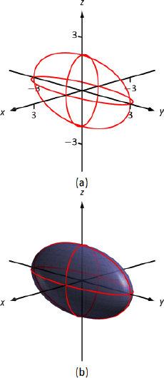
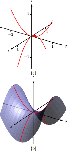
   Figure \(\PageIndex{15}\): Sketching an ellipsoid.
3. \( z=y^2-x^2\):
   
   This defines a hyperbolic paraboloid, very similar to the one shown in the gallery of quadric sections. Consider the traces in the \(y-z\) and \(x-z\) planes:
   
   \(x=0\): The trace is \(z=y^2\), a parabola opening up in the \(y-z\) plane.
   
   \(y=0\): The trace is \(z=-x^2\), a parabola opening down in the \(x-z\) plane.
   
   Sketching these two parabolas gives a sketch like that in Figure Figure \(\PageIndex{16a}\), and filling in the surface gives a sketch like Figure \(\PageIndex{16b}\).

Figure \(\PageIndex{16}\): Sketching a hyperbolic paraboloid.

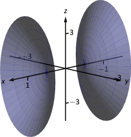
Example \(\PageIndex{8}\): Identifying quadric surfaces

Consider the quadric surface shown in Figure Figure \(\PageIndex{17}\). Which of the following equations best fits this surface?

Figure \(\PageIndex{8}\).

\[\nonumber \begin{align}
(a)\, & x^2-y^2-\frac{z^2}{9}=0\qquad\qquad && (c) \, z^2-x^2-y^2=1 \\ \nonumber
(b)\, & x^2-y^2-z^2=1 \qquad\qquad && (d) \, 4x^2-y^2-\frac{z^2}9=1
\end{align}\]

Solution

The image clearly displays a hyperboloid of two sheets. The gallery informs us that the equation will have a form similar to \(\frac{z^2}{c^2}-\frac{x^2}{a^2}-\frac{y^2}{b^2}=1\).

We can immediately eliminate option (a), as the constant in that equation is not 1.

The hyperboloid "opens'' along the \(x\)-axis, meaning \(x\) must be the only variable with a positive coefficient, eliminating (c).

The hyperboloid is wider in the \(z\)-direction than in the \(y\)-direction, so we need an equation where \(c>b\). This eliminates (b), leaving us with (d). We should verify that the equation given in (d), \(4x^2-y^2-\frac{z^2}9=1\), fits.

We already established that this equation describes a hyperboloid of two sheets that opens in the \(x\)-direction and is wider in the \(z\)-direction than in the \(y\). Now note the coefficient of the \(x\)-term. Rewriting \(4x^2\) in standard form, we have: \( 4x^2 = \frac{x^2}{(1/2)^2}\). Thus when \(y=0\) and \(z=0\), \(x\) must be \(1/2\); i.e., each hyperboloid "starts'' at \(x=1/2\). This matches our figure.

We conclude that \( 4x^2-y^2-\frac{z^2}9=1\) best fits the graph.

This section has introduced points in space and shown how equations can describe surfaces. The next sections explore vectors, an important mathematical object that we'll use to explore curves in space.

Contributors and Attributions

• Gregory Hartman (Virginia Military Institute). Contributions were made by Troy Siemers and Dimplekumar Chalishajar of VMI and Brian Heinold of Mount Saint Mary's University. This content is copyrighted by a Creative Commons Attribution - Noncommercial (BY-NC) License. http://www.apexcalculus.com/